guide
This article is compiled from the topic sharing of the same name on the topic of AI infrastructure at the QCon Global Software Development Conference (Beijing Station) in February 2023. Applications such as ChatGPT, Bard and the "Wen Xin Yi Yan" that will meet with you are all based on the large models launched by each manufacturer. GPT-3 has 175 billion parameters, and Wenxin large model has 260 billion parameters. Taking the use of NVIDIA GPU A100 to train GPT-3 as an example, theoretically, it takes 32 years for a single card, and a distributed cluster with a kilocalorie scale, after various optimizations, still needs 34 days to complete the training. This speech introduced the challenges of large-scale model training to infrastructure, such as computing power walls, storage walls, single-machine and cluster high-performance network design, graph access and back-end acceleration, model splitting and mapping, etc., shared Baidu The response method and engineering practice of the intelligent cloud have built a full-stack infrastructure from the framework to the cluster, combining software and hardware, and accelerated the end-to-end training of large models.
In the past two years, the big model has had the greatest impact on the AI technology architecture. In the process of large model generation, iteration and evolution, it poses new challenges to the underlying infrastructure.
Today's sharing is mainly divided into four parts. The first part is to introduce the key changes brought about by the big model from a business perspective. The second part is about the challenges that large model training poses to infrastructure in the era of large models and how Baidu Smart Cloud responds. The third part is to combine the needs of large-scale models and platform construction, and explain the joint optimization of software and hardware made by Baidu Smart Cloud. The fourth part is Baidu Smart Cloud's thoughts on the future development of large models and new requirements for infrastructure.
1. GPT-3 opens the era of large models
The era of large models was opened by GPT-3, which has the following characteristics:
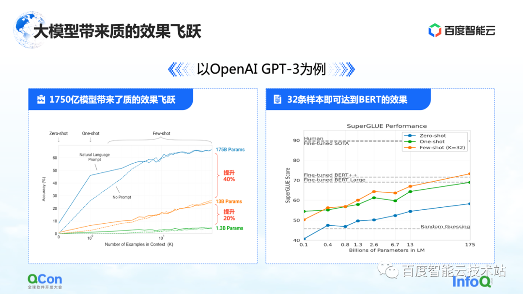
The first feature is that the parameters of the model have been greatly improved. A single model has reached 175 billion parameters, which has also brought about a significant increase in accuracy. From the figure on the left, we can see that with more and more model parameters, the accuracy of the model is also improving.
The picture on the right shows its more shocking features: based on the pre-trained 175 billion parameter model, it only needs to be trained with a small number of samples, and it can approach the effect of BERT after using large sample training. This reflects to a certain extent that the scale of the model becomes larger, which can bring about improvements in model performance and model versatility.
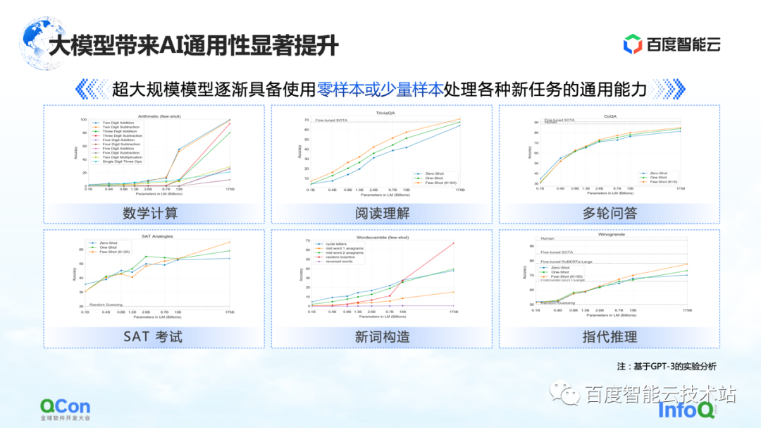
In addition, GPT-3 also shows a certain degree of versatility in tasks such as mathematical calculations, reading comprehension, and multiple rounds of question and answer. Only a small number of samples can make the model achieve higher accuracy, even close to human accuracy. Spend.
Because of this, the large model has also brought new changes to the overall AI research and development model. In the future, we may pre-train a large model first, and then perform Fine-tune with a small number of samples for specific tasks to obtain good training results. Instead of training the model like now, each task needs to be completely iterated and trained from scratch.
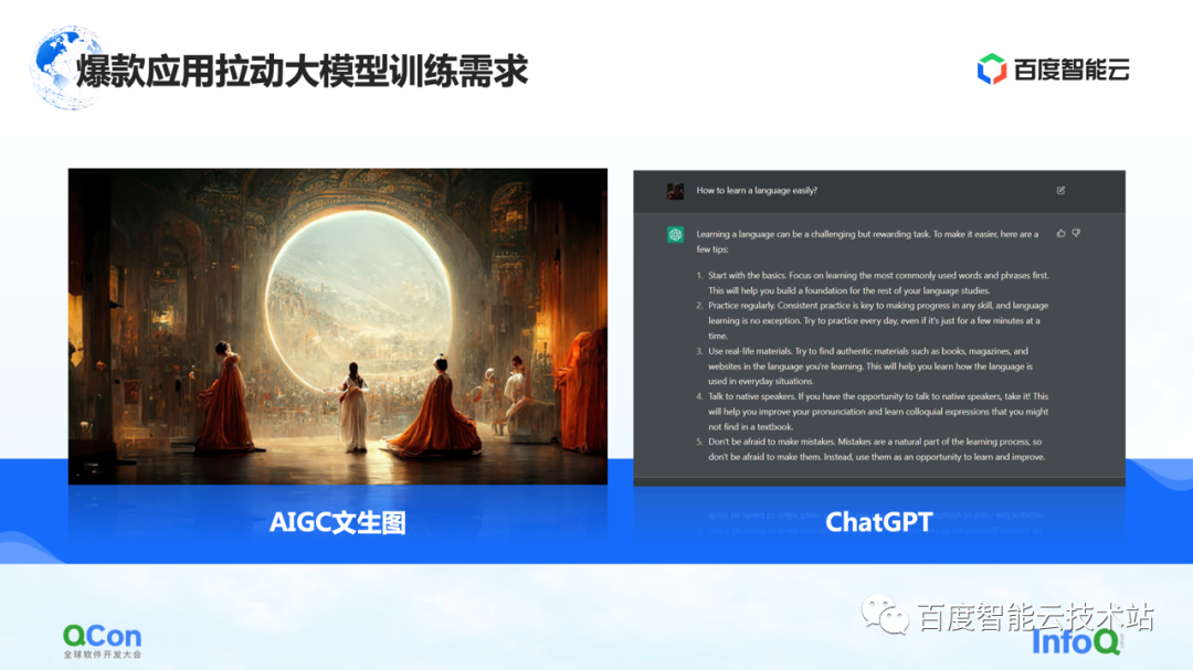
Baidu started training large models very early, and the Wenxin large model with 260 billion parameters was released in 2021. Now with Stable Diffusion, AIGC Vincent graph, and the recently popular chat robot ChatGPT, etc., which have attracted the attention of the whole society, everyone really realizes that the era of large models has arrived.
Manufacturers are also laying out products related to large models. Google has just released Bard before, and Baidu will soon launch "Wen Xin Yi Yan" in March.
What are the different characteristics of large model training?
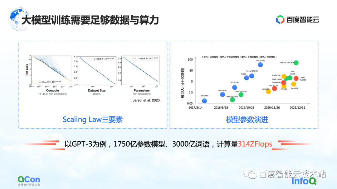
The large model has a Scaling Law, as shown in the figure on the left, as the model's parameter scale and training data increase, the effect will become better and better.
But there is a premise here, the parameters must be large enough, and the data set is sufficient to support the training of the entire parameter. The consequence of this is that the amount of calculations increases exponentially. For an ordinary small model, a single machine and a single card can be done. But for a large model, its requirements for training volume require large-scale resources to support its training.
Taking GPT-3 as an example, it is a model with 175 billion parameters and needs 300 billion words of training to support it to achieve a good effect. Its calculation is estimated to be 314 ZFLOPs in the paper. Compared with NVIDIA GPU A100, a card is still only 312 TFLOPS AI computing power, and the absolute value in the middle is different by 9 orders of magnitude.
Therefore, in order to better support the calculation, training and evolution of large models, how to design and develop infrastructure has become a very important issue.
2. Large-scale model infrastructure panorama
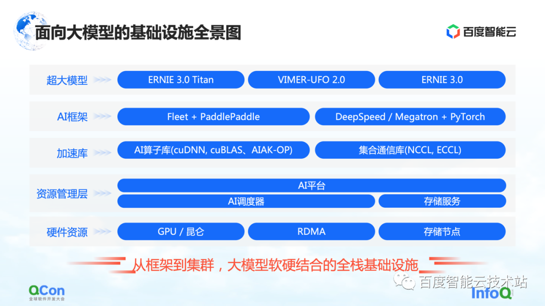
This is a panorama of Baidu Smart Cloud's infrastructure for large models. This is a full-stack infrastructure covering from framework to cluster, combining hardware and software.
In the large model, infrastructure no longer only covers traditional infrastructure such as underlying hardware and networks. We also need to bring all relevant resources into the category of infrastructure.
Specifically, it is roughly divided into several levels:
-
The top layer is the model layer, including internal and external published models and some supporting components. For example, Baidu's flying paddle PaddlePaddle and Fleet, Fleet is a distributed strategy on the flying paddle . At the same time, in the open source community, such as PyTorch, there are some large-scale model training frameworks and acceleration capabilities based on the PyTorch framework, such as DeepSpeed/Megatron.
-
Under the framework, we will also develop related capabilities of the acceleration library, including AI operator acceleration, communication acceleration, etc.
-
The following are some related capabilities of partial resource management or partial cluster management.
-
At the bottom are hardware resources, such as stand-alone single-card, heterogeneous chips, and network-related capabilities.
The above is a panorama of the entire infrastructure. Today I will focus on starting with the AI framework, and then extend to the acceleration layer and hardware layer to share some specific work of Baidu Smart Cloud.
Start with the top AI framework first.
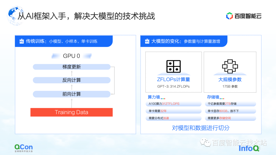
For the traditional small model training on a single card, we can complete the entire training by using the training data to continuously update the forward and reverse gradients. For the training of large models, there are two main challenges: the computing power wall and the storage wall.
The computing power wall refers to how we can use distributed methods to break the problem of too long time for single computing power if we want to complete the model training of GPT-3, which requires 314 ZFLOPs computing power, but the single card only has 312 TFLOPS computing power. . After all, it takes 32 years to train a model with one card, which is obviously not feasible.
Next is the storage wall. This is a bigger challenge for larger models. When a single card cannot hold the model, the model must have some method of segmentation.
For example, the storage of a 100-billion-level large model (including parameters, training intermediate values, etc.) requires 2 TB of storage space, while the maximum video memory of a single card is currently only 80 GB. Therefore, the training of large models requires some segmentation strategies to solve the problem that a single card cannot fit.
The first is the computing power wall, which solves the problem of insufficient computing power of a single card.
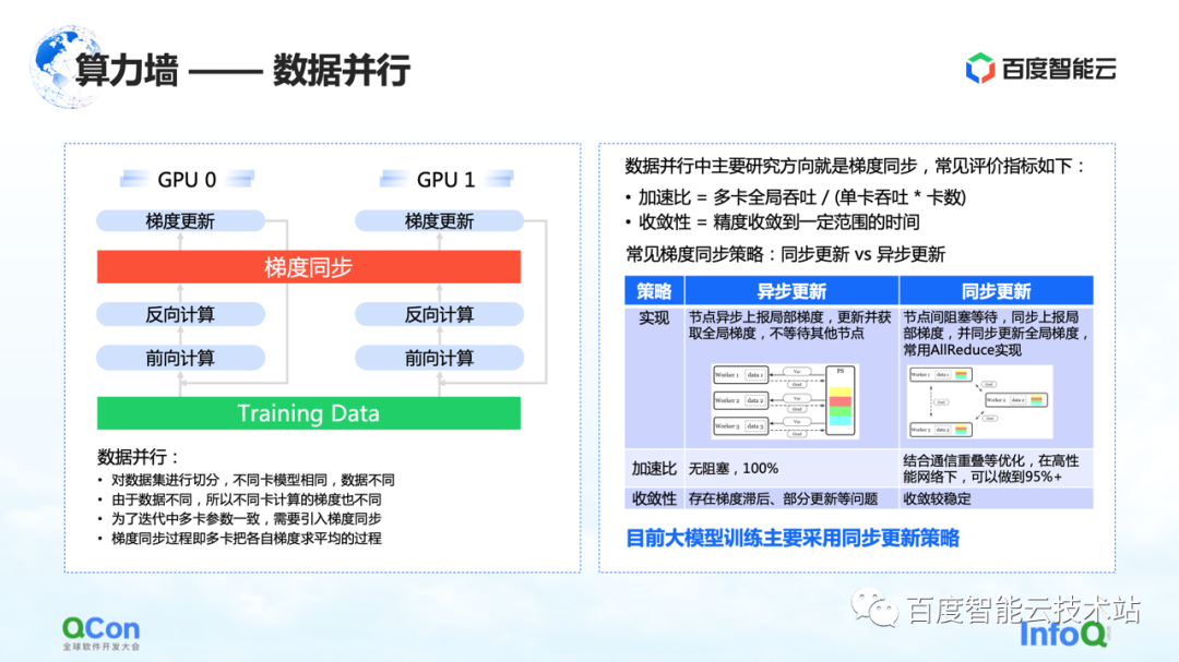
A very simple and most familiar idea is data parallelism, which cuts training samples to different cards. Overall, the large model training process we are observing now mainly adopts a synchronous data update strategy.
The focus is on the solution to the storage wall problem. The key is the strategy and method of model segmentation.
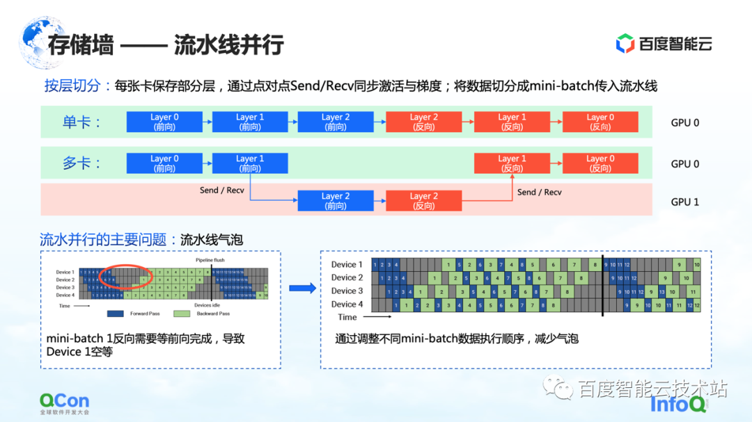
The first slicing method is pipelined parallelism.
Let's use the example in the figure below to illustrate. For a model, it is composed of many layers. When training, do forward first and then reverse. For example, the three layers 0, 1, and 2 in the picture cannot fit on one card. After we divide by layer, we will put some layers in this model on the first card. For example, in the figure below, the green area represents GPU 0, and the red area represents GPU 1. We can put the first few layers on GPU 0 and the other few layers on GPU 1. When the data is flowing, it will first do two forwards on GPU 0, then do one forward and one reverse on GPU 1, and then return to GPU 0 to do two reverses. Since this process is particularly pipeline-like, we call it pipeline parallelism.
But there is a major problem with pipeline parallelism, namely pipeline bubbles. Because there will be dependencies between the data, and the gradient depends on the calculation of the previous layer, so in the process of data flow, bubbles will be generated, which will cause emptiness. In response to such problems, we reduce the empty time of bubbles by adjusting the execution strategies of different mini-batches.
The above is the perspective of an algorithm engineer or a framework engineer to look at this problem. From the perspective of infrastructure engineers, we are more concerned about the different changes it will bring to the infrastructure.
Here we focus on its communication semantics. It is between forward and backward, and it needs to pass its own activation value and gradient value, which will bring additional Send/Receive operations. And Send/Receive is point-to-point, we will mention the solution later in the article.
The above is the first parallel model segmentation strategy that breaks the storage wall: pipeline parallelism.
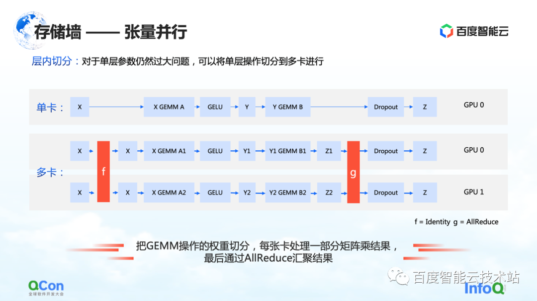
The second segmentation method is tensor parallelism , which solves the problem of too large single-layer parameters.
Although the model has many layers, one of the layers is computationally intensive. At this time, we expect the calculation amount of this layer to be jointly calculated between machines or between cards. From the perspective of an algorithm engineer, the solution is to divide different inputs into several pieces, then use different pieces to perform partial calculations, and finally perform aggregation.
But from the perspective of infrastructure engineers, we still pay attention to what additional operations are introduced in this process. In the scenario just mentioned, the extra operations are f and g in the graph. What do f and g stand for? When doing forward, f is an invariant operation, and x is transparently transmitted through f, and some calculations can be done later. However, when the results are aggregated at the end, the entire value needs to be passed down. For this case, it is necessary to introduce the operation of g. g is the operation of AllReduce, which semantically aggregates two different values to ensure that the output z can get the same data on both cards.
So from the perspective of infrastructure engineers, you will see that it introduces additional AllReduce communication operations. The communication traffic of this operation is still relatively large, because the parameters in it are relatively large. We will also mention the method of coping later in the article
This is the second optimization method that can break storage walls.
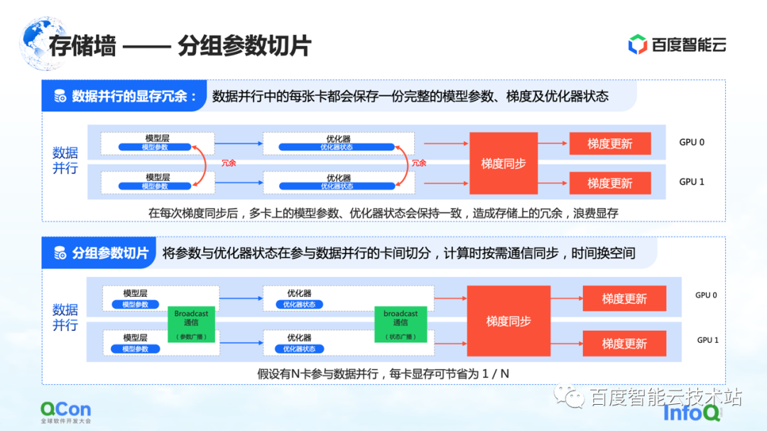
The third method of slicing is grouped parameter slicing . This method reduces the memory redundancy in data parallelism to a certain extent. In traditional data runs, each card will have its own model parameters and optimizer state. Since they need to be synchronized and updated during their respective training processes, these states are fully backed up on different cards,
For the above process, in fact, the same data and parameters are stored redundantly on different cards. Such redundant storage is unacceptable because large models have extremely high storage space requirements. In order to solve this problem, we split the model parameters and only keep a part of the parameters on each card.
When calculations are really needed, we trade time for space: first synchronize the parameters, and then discard the redundant data after the calculation is completed. In this way, the demand for video memory can be further compressed, and training can be better performed on existing machines.
Similarly, from the perspective of infrastructure engineers, we need to introduce communication operations such as broadcast, and the communication content is the state of these optimizers and the parameters of the model.
The above is the third optimization method to break the storage wall.
In addition to the memory optimization methods and strategies mentioned above, there is another way to reduce the amount of calculation of the model.
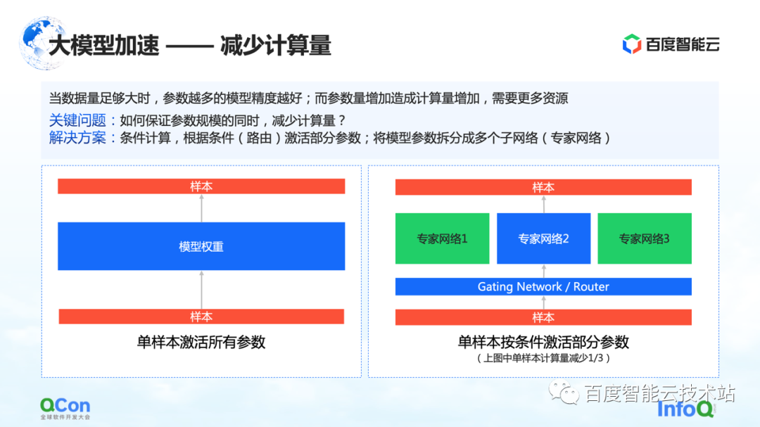
When the amount of data is large enough, the more parameters of the model, the better the accuracy of the model. However, with the increase of parameters, the amount of calculation also increases, requiring more resources, and at the same time, the calculation time will be longer.
So how to ensure that the amount of calculation is reduced while the parameter scale remains unchanged? One of the solutions is conditional computing: according to certain conditions (that is, the Gating layer in the figure on the right, or called the routing layer), to select and activate some of the parameters.
For example, in the figure on the right, we divide the parameters into three parts, and according to the conditions of the model, only part of the parameters are activated for calculation in the expert network 2. Some parameters in expert 1 and expert 3 are not calculated. In this way, the calculation amount can be reduced while ensuring the parameter scale.
The above is a method based on conditional calculation to reduce the amount of calculation.
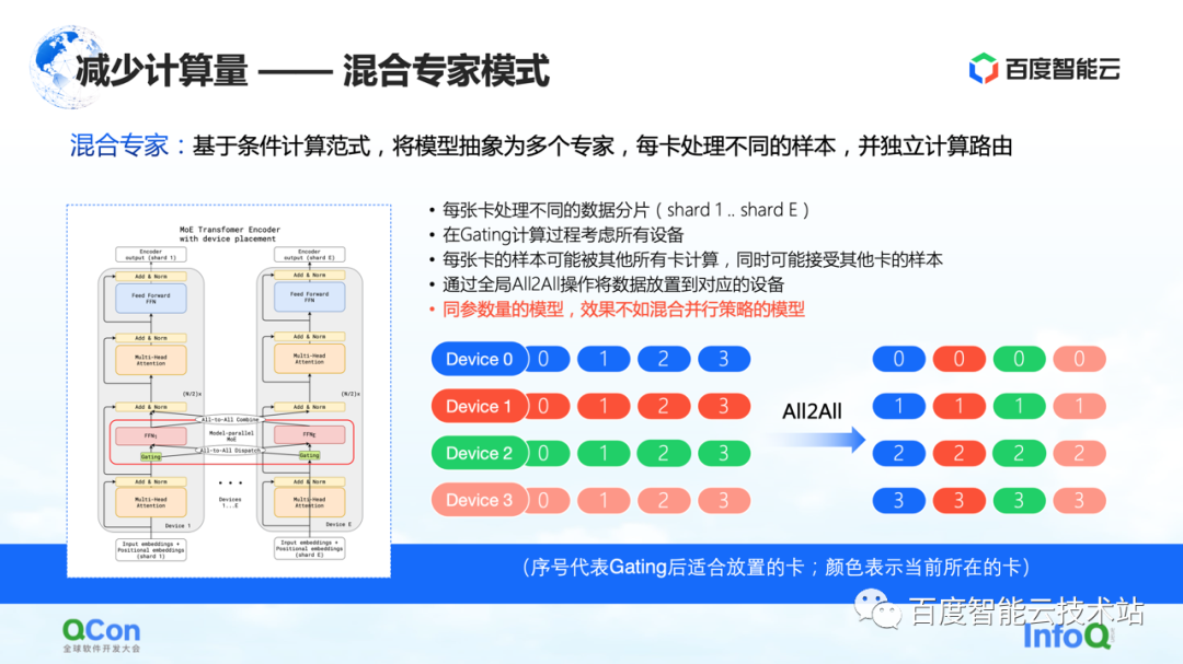
Based on the above method, the industry proposed a mixed-expert model , which is to abstract the model into multiple experts, and each card processes different samples. Specifically, some routing choices are inserted in the model layer, and then only some of the parameters are activated according to this choice. At the same time, the parameters of different experts will be kept on different cards. In this way, in the process of sample distribution, they will be allocated to different cards for calculation.
But from the perspective of an infrastructure engineer, we found that the All2All operation was introduced in this process. As shown in the right figure below, samples such as 0, 1, 2, and 3 are stored on multiple Devices. The value in Device indicates which card is suitable for calculation, or which expert it is suitable for calculation. For example, 0 means that it is suitable to be calculated by No. 0 expert, that is, No. 0 card, and so on. Each card will determine who is suitable for the stored data to be calculated. For example, card No. 1 judges that some parameters are suitable for calculation by No. 0 card, and other parameters are suitable for calculation by No. 1 card. Then the next action is to distribute the samples to different cards.
After the above operations, the samples on the No. 0 card are all 0s, and the samples on the No. 1 card are all 1s. The above process is called All2All in communication. From the perspective of infrastructure engineers, this operation is a relatively heavy operation, and we need to make some related optimizations on this basis. We will also introduce further in the following text.
In this mode, one of the phenomena we observed is that if the mixed-expert mode is used, its training accuracy is not as good as the various parallel strategies and hybrid superposition strategies mentioned just now under the model of the same parameters. Choose according to the actual situation.
I just introduced several parallel strategies, and then I will share an internal practice of Baidu Smart Cloud.
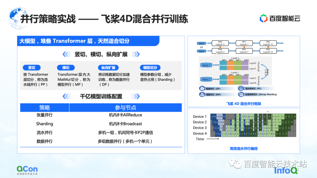
We trained a large model with 260 billion parameters using Paddle , stacking some layers of optimized Transformer classes. We can slice it horizontally and vertically. For example, vertically slice the model according to the Transformer layer using the pipeline parallel strategy. Cross-cutting is to use the model parallel strategy/tensor parallel strategy to split the calculation of large matrix multiplication such as MetaMul inside Transformer. At the same time, we supplemented it with vertical optimization of data parallelism and video memory optimization of grouping model parameter segmentation in data parallelism. Through the above four methods, we introduced the framework of 4D hybrid parallel training of flying paddles .
In the training configuration of the 100 billion parameter model, we use eight cards in the machine to do tensor parallelism, and at the same time cooperate with data parallelism to perform some grouping parameter segmentation operations. At the same time, multiple groups of machines are used to form a parallel pipeline to carry 260 billion model parameters. Finally, the data parallel method is used for distributed computing to complete the monthly training of the model.
The above is an actual combat of our entire model parallel parameter model parallel strategy.
Next, let us return to the perspective of infrastructure to evaluate the communication and computing power requirements of different segmentation strategies in model training.
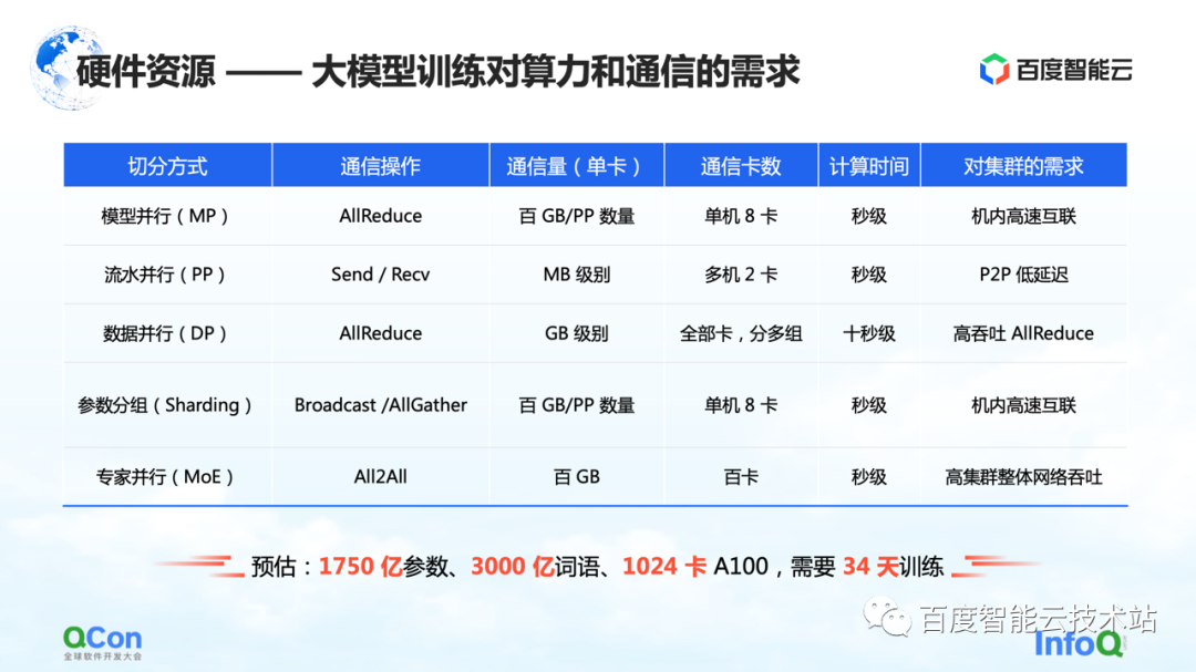
As shown in the table, we list the communication traffic and computing time required for different segmentation methods according to the scale of 100 billion parameters. From the perspective of the entire training process, the best effect is that the calculation process and the communication process can be completely covered or overlapped with each other.
From this table, we can deduce the requirements of the 100 billion parameter model for clusters, hardware, networks, and overall communication modes. Based on a model with an estimated 175 billion parameters trained on 1024 A100 cards using 300 billion words, it takes 34 days to complete the full end-to-end training.
The above is our evaluation of the hardware side.
With the hardware requirements, the next step is the selection of stand-alone and network levels.
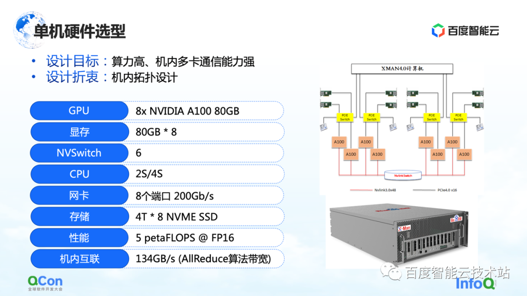
At the stand-alone level, since a large number of AllReduce and Broadcast operations need to be performed in the machine, we hope that the machine can support high-performance, high-bandwidth connections. So we used the most advanced A100 80G package in the model selection at that time, using 8 A100s to form a single machine.
In addition, in the external network connection method, the most important thing is the topology connection method. We hope that the network card and the GPU card can be under the same PCIe Switch as much as possible, and the throughput bottleneck of the interaction between the cards during the entire training process can be better reduced in a symmetrical way. At the same time, try to avoid them passing through the PCIe Root Port of the CPU.
After talking about the stand-alone, let's take a look at the design of the cluster network.
First of all, let's evaluate the requirements. If our business expectation is to complete the end-to-end model training within one month, we need to reach the kilocalorie level in single-job training, and the 10,000-calorie level in large model training clusters. Therefore, in the process of network design, we should take into account two points:
First, in order to meet the point-to-point operation of Send/Receive in the pipeline, it is necessary to reduce the P2P delay.
Second, since the network-side traffic in AI training is concentrated on the AllReduce operation of the same card, we also hope that it has a high communication throughput.
for this communication need. We designed the topology of the three-tier CLOS architecture shown on the right. Compared with the traditional method, the most important thing about this topology is the optimization of the eight guide rails, so that the number of jumps in the communication of any card with the same number in different machines is as small as possible.
In the CLOS architecture, the bottom layer is Unit. There are 20 machines in each Unit, and we connect the GPU cards of the same number in each machine to the same group of TORs with corresponding numbers. In this way, all cards of the same number in a single unit can complete the communication with only one hop, which can greatly improve the communication between cards of the same number.
However, there are only 20 machines with a total of 160 cards in one unit, which cannot meet the requirements for large model training. So we designed the second layer Leaf layer. The Leaf layer connects cards with the same number in different units to the switching devices of the same group of Leafs, which still solves the problem of interconnecting cards with the same number. Through this layer, we can interconnect 20 Units again. So far, we have been able to connect 400 machines with a total of 3200 cards. For such a 3200-card cluster, communication between any two cards of the same number can be realized by hopping up to 3 hops.
What if we want to support the communication of cards with different numbers? We added a Spine layer on top to solve the problem of communication between cards with different numbers.
Through this three-layer architecture, we have realized an overall architecture that supports 3200 cards optimized for AllReduce operations. If it is on the network equipment of IB, the architecture can support the scale of 16000 cards, which is also the largest scale of IB box-type networking at present.
We compared the CLOS architecture with some other network architectures, such as Dragonfly, Torus, etc. Compared with them, the network bandwidth of this architecture is more sufficient, and the number of hops between nodes is more stable, which is very helpful for estimating predictable training performance.
The above is a set of construction ideas from stand-alone to cluster network.

3. Joint optimization of the combination of software and hardware
Large-scale model training does not mean buying the hardware and putting it there to complete the training. We also need joint optimization of hardware and software.
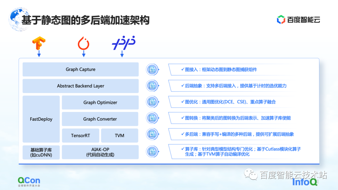
First of all, let's talk about calculation optimization. The training of large models is still a computationally intensive process as a whole. In terms of computing optimization, many current ideas and ideas are based on multi-backend acceleration of static graphs. The graphs constructed by users, whether it is Paddle , PyTorch or TensorFlow, will first convert the dynamic graphs into static graphs through graph capture, and then let the static graphs enter the backend for acceleration.
The figure below shows our entire static graph-based multi-backend architecture, which is divided into the following parts**. **
The first is graph access, which converts dynamic graphs into static graphs.
The second is the multi-backend access method, which provides timing-based optimization capabilities through different backends.
The third is graph optimization. We have done some calculation optimization and graph conversion for static graphs, so as to further improve computing efficiency.
Finally, we will use some custom operators to speed up the training process of the large model as a whole.
Let's introduce them separately below.
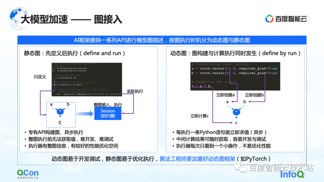
In the training architecture of large models, the first part is graph access. When describing graphs in the AI framework, they are usually divided into static graphs and dynamic graphs.
The static graph is that the user constructs the graph before executing it, and then executes it in combination with his actual input. Combined with such characteristics, some compilation optimization or scheduling optimization can be done in advance during the calculation process, which can better improve the training performance.
But corresponding to it is the construction process of the dynamic graph. The user writes some code casually, and it is dynamically executed during the writing process. For example, PyTorch, after the user writes a statement, it will perform related execution and evaluation. For users, the advantage of this approach is that it is easy to develop and debug. But for the executor or the acceleration process, because each time it is seen is a small part of the operation, it is not very well optimized.
In order to solve this problem, the general idea is to integrate dynamic graphs and static graphs, use dynamic graphs for development, and then execute through static graphs. There are mainly two paths to implementation that we see now.
The first is to do static conversion based on Python AST. For example, we get the Python source code written by the user, convert it into a Python AST tree, and then do CodeGen based on the AST tree. In this process, the dynamic source code of Python can be converted into a static graph by using the method and API of static group graph.
But in this process, the biggest problem is the flexibility of the Python language, which leads to the inability of static analysis to understand the semantics well, and then the conversion of dynamic images to static images fails. For example, in the process of static analysis, it has no way to infer the dynamic type, and for example, the static analysis cannot infer the range of the range, resulting in frequent failures in the actual conversion process. So static conversion can only be applied to some simple model scenarios.
The second route is to do simple execution and simulation by means of Tracing or Symbolic Tracing. Tracer records some computing nodes encountered during the recording process. After recording these computing nodes, it constructs an entire static graph a posteriori through playback or reorganization. The advantage of this method is that it can capture and calculate the overall dynamic graph by simulating some input methods, or by constructing special structure methods, and then can capture a path more successfully.
But there are actually some problems in this process. For branch or loop structures that depend on input, because Tracer constructs static graphs by constructing simulated inputs, Tracer will only go to some of the branches, which leads to security problems.
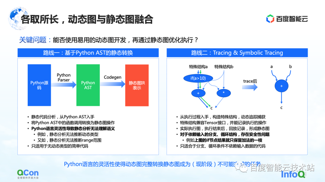
After comparing these methods, we found that under the existing language flexibility of Python, it is basically an impossible task to complete the conversion of dynamic graphs into static graphs at this stage. Therefore, our focus has shifted to how to provide users with more secure and easy-to-use image conversion capabilities on the cloud. At this stage, there are several options as follows.
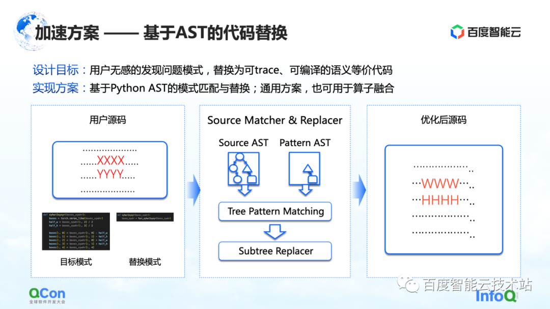
The first solution is to develop a method based on AST code replacement. In this method, Baidu Smart Cloud provides the corresponding model conversion and optimization capabilities, which is insensitive to users. For example, the user enters a piece of source code, but some of the code (shown as XXXX and YYYY in the figure) is in the process of static image capture, graph optimization, and operator optimization. We found that this part of the code cannot convert the dynamic graph into a static graph. Or the code has room for performance optimization. Then we will write a replacement code, as shown in the middle picture. On the left is a piece of Python code that we think can be replaced, and on the right is another piece of Python code that we have replaced. Then, we will use the AST matching method to convert the user's input and our original target pattern into AST, and execute our subtree tree matching algorithm on it.
In this way, we can change our original input XXXX, YYYY into WWWW, HHHH, and turn it into a solution that can be executed better, which improves the success rate of converting dynamic images to static images to a certain extent, and improves the operator at the same time. performance, and can achieve the effect that the user is basically insensitive.
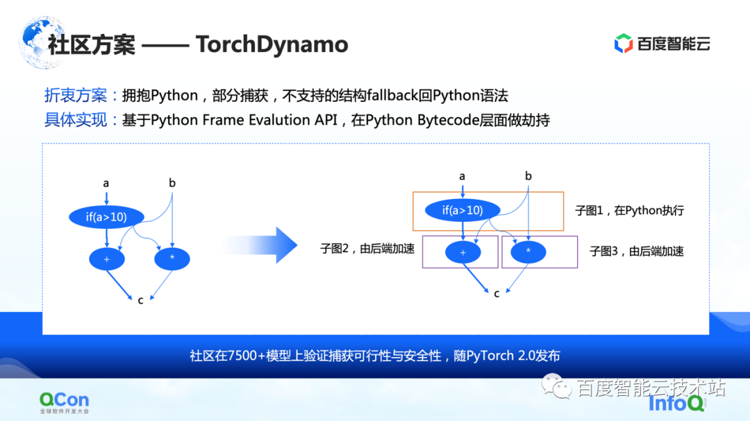
The second is some solutions in the community, especially the TorchDynamo solution proposed by PyTorch 2.0, which is also a solution that we have seen so far that is more suitable for computing optimization. It can achieve partial graph capture, and unsupported structures can fallback back to Python. In this way, it can spit out some of the subgraphs to the backend to a certain extent, and then the backend can further accelerate calculations on these subgraphs.
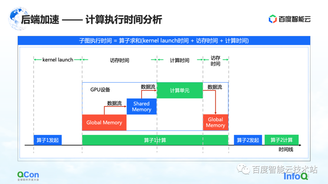
After we have captured the entire graph, the next step is to actually start computing acceleration, that is, back-end acceleration.
We believe that the key points in the timing diagram of GPU computing are memory access time and computing time. We accelerate this time from the following angles.
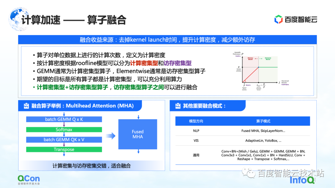
The first one is operator fusion. The main benefit of operator fusion is to reduce the time spent on kernel launch, increase computing density, and reduce additional memory access. We define the number of calculations per unit memory access of an operator as the calculation density.
According to the difference in computing density, we divide operators into two types: computing-intensive and memory-intensive. For example, GEMM is a typical computation-intensive operator, and Elementwise is a typical memory-intensive operator. We found that a good fusion can be made between "computation-intensive operators + memory-intensive operators" and "memory-intensive operators + memory-intensive operators".
Our goal is to convert all the operators executed on the GPU into partial calculation-intensive operators, so that we can make full use of our computing power.
On the left is an example of ours. For example, in the Transformer structure, the most important Multihead Attention can do a good fusion. At the same time, there are some other models that we found on the right, and we will not list them one by one due to space limitations.
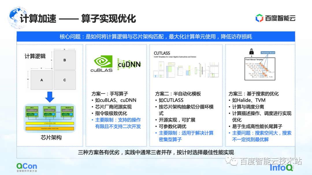
Another type of computing optimization is the optimization of operator implementation.
The essential issue of operator implementation is how to combine computing logic with chip architecture, so as to better realize the entire computing process. We currently see three types of scenarios:
The first category is handwritten operators. Relevant manufacturers will provide operator libraries such as cuBLAS and cuDNN. The operator performance it provides is the best, but the operations it supports are limited, and the support for custom development is relatively poor.
The second category is semi-automated templates, such as CUTLASS. This method makes an open source abstraction, allowing developers to do secondary development on it. This is also the method we currently use to achieve the fusion of computation-intensive and memory-intensive operators.
The third is search-based optimization. We paid attention to some compiling methods like Halide and TVM in the community. At present, it is found that this method is effective on some operators, but it needs further polishing on other operators.
In practice, these three methods have their own advantages, so we will provide you with the best implementation through timing selection.
After talking about the optimization of computing, let's share several methods of communication optimization.
The first is the resolution of the switch hash collision problem. The figure below is an experiment we did. We set up a 32-card task and performed 30 AllReduce operations each time. The figure below shows the communication bandwidth we measured. We can see that there is a high probability that it will slow down. This is a serious problem in large model training.
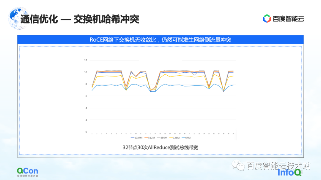
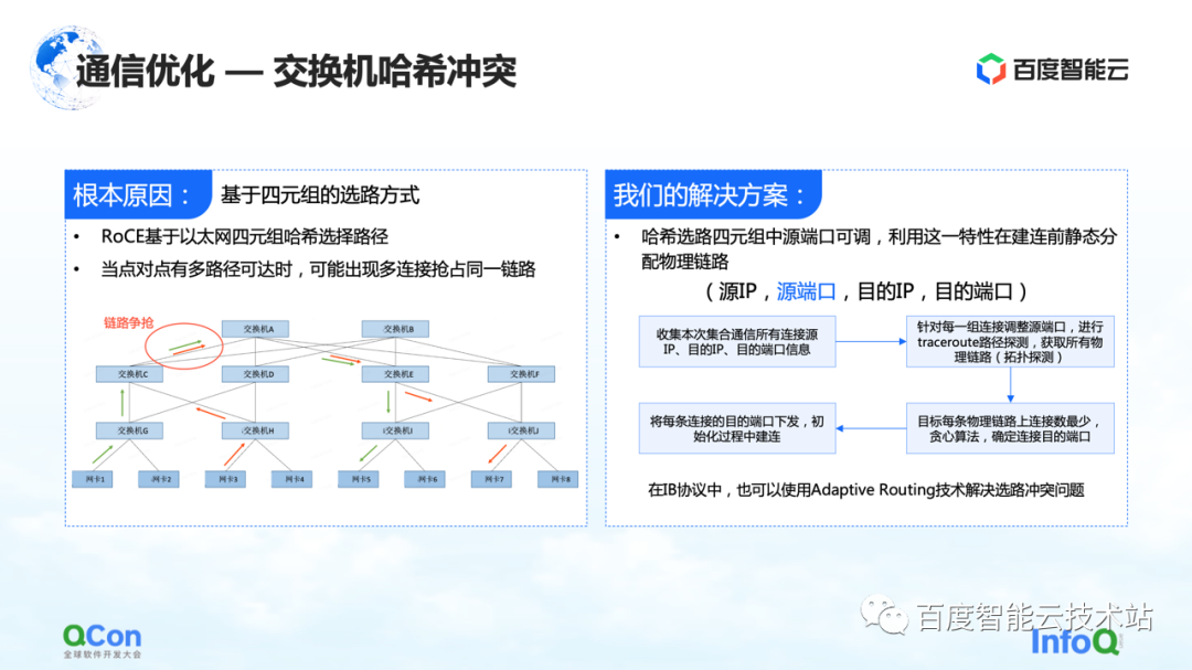
The reason for the slowdown is because of hash collisions. Although in the network design, the switch has no convergence ratio, that is, the bandwidth resources in our network design are sufficient, but due to the use of RoCE, a method based on Ethernet quadruple routing, traffic conflicts on the network side may still occur .
For example, in the example in the figure below, the green machines need to communicate with each other, and the red machines also need to communicate with each other. Then during the route selection process, everyone’s communication will compete for the same bandwidth due to hash conflicts, resulting in Although the overall network bandwidth is sufficient, local network hotspots will still form, resulting in a slowdown in communication performance.
Our solution is actually quite simple. In the whole communication process, there are four tuples of source IP, source port, destination IP and destination port. The source IP, destination IP, and destination port are fixed, while the source port can be adjusted. Taking advantage of this feature, we continuously adjust the source port to select different paths, and then use the overall greedy algorithm to minimize the occurrence of hash collisions.
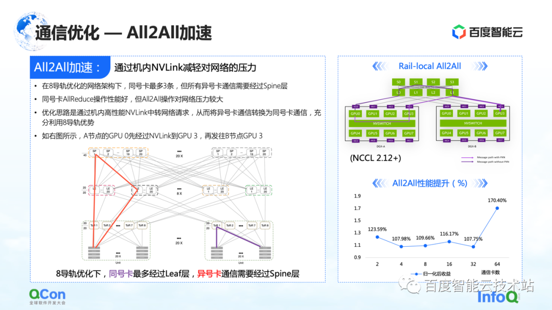
In communication optimization, in addition to some optimizations on AllReduce just mentioned, there is also a certain room for optimization on All2All, especially our specially customized network for eight rails.
This network will put a lot of pressure on the upper layer spine switch in the operation of the whole All2All. The optimization method is to use the Rail-Local All2All in NCCL, or the optimization of PXN. The principle is to convert the communication between cards of different numbers to the communication between cards of the same number through the high-performance NVLink inside the machine.
In this way, we convert all the network communication between machines that originally went up to the spine layer into intra-machine communication, so that only the TOR layer or leaf layer communication can be used to realize the communication of cards with different numbers, and the performance will also be improved. There is a big improvement.
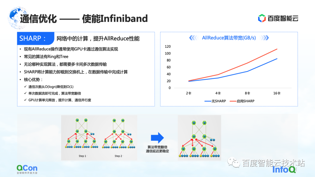
In addition, in addition to these optimizations done on RoCE, there is another direct effect that can be achieved by enabling Infiniband. For example, the switch hash conflict just mentioned can be handled by its own adaptive routing. For AllReduce, it also has some advanced features such as Sharp, which can well offload part of AllReduce computing operations to our network devices, so as to release computing units and improve computing performance. Through this method, we can well improve the training effect of AllReduce again.
Just finished talking about the optimization of computing and communication, let's look at this problem from end to end.
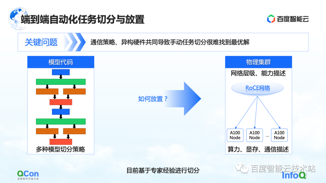
From the perspective of the entire large model training, it is actually divided into two parts, the first part is the model code, and the second part is the high-performance network. At these two different levels, there is a problem to be solved urgently: which card is the most appropriate to place the model after multiple segmentation strategies?
Let's take an example. When doing tensor parallelism, we need to divide the calculation of a tensor into two parts. Since a large number of AllReduce operations are required between the calculation results of the blocks, a high bandwidth is required.
If we put two pieces of a tensor cut in parallel on two cards of different machines, network communication will be introduced, causing performance problems. On the contrary, if we put these two pieces in the same machine, we can efficiently complete the computing tasks and improve the training efficiency. Therefore, the core appeal of the placement problem is to find the most suitable or best-performing mapping relationship between the segmented model and heterogeneous hardware.
In our early model training, the mapping was done manually based on expert empirical knowledge. For example, the picture below shows that when we cooperate with the business team, when we think that the bandwidth in the machine is good, we recommend putting it in the machine. If we think that there may be improvements in the machine room, it is recommended to put it in the machine room.
Is there any engineering or systematic solution?
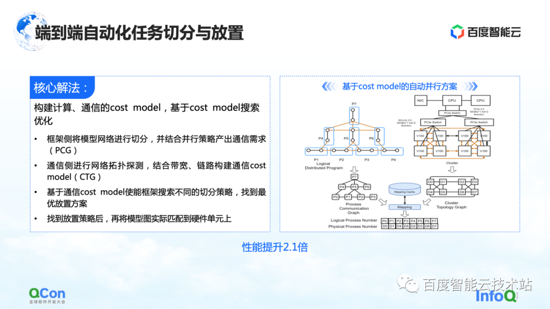
Our core solution is to build a cost model for computing and communication, and then do search optimization based on the cost model. In this way an optimal mapping is produced.
In the whole process, the model network on the framework side will be abstracted and segmented first, and mapped into a computing framework diagram. At the same time, the computing and communication capabilities of the stand-alone and the cluster will be modeled to create a topology map of the cluster.
When we have the computing and communication requirements on the model on the left side of the right picture, and the computing and communication capabilities on the hardware on the right side of the picture, we can split and map the model through graph algorithms or other search methods, and finally get An optimal solution at the bottom of the figure on the right.
In the actual large model training process, the final performance can be improved by 2.1 times in this way.
4. The development of large models promotes the evolution of infrastructure
Finally, I will discuss with you what new requirements the large model will put on infrastructure in the future.
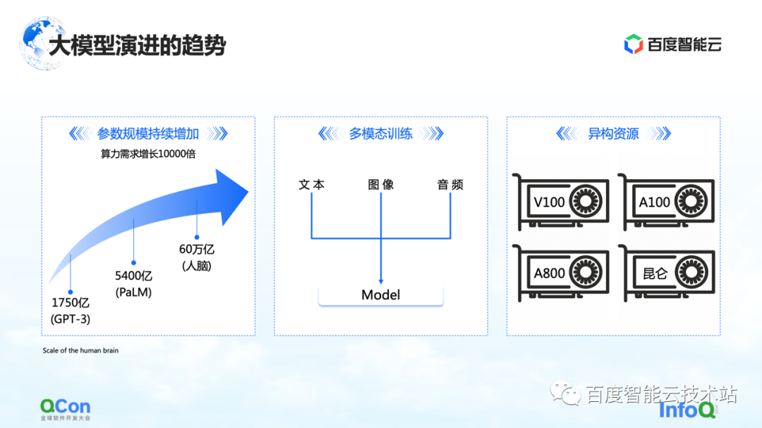
There are three changes we are seeing so far. The first is the parameters of the model, and the model parameters will continue to grow, from 175 billion in GPT-3 to 540 billion in PaLM. Regarding the final value of future parameter growth, we can refer to the human brain with a scale of about 60 trillion parameters.
The second is multimodal training. In the future we will deal with more modal data. Different modal data will bring more challenges to storage, computation, and video memory.
The third is heterogeneous resources. In the future we will have more and more heterogeneous resources. In the training process, various types of computing power, how to better use them is also an urgent challenge to be solved.
At the same time, from a business perspective, there may be different types of jobs in a complete training process, and there may be traditional GPT-3 training, reinforcement learning training, and data labeling tasks at the same time. How to better place these heterogeneous tasks on our heterogeneous cluster will be a bigger problem.
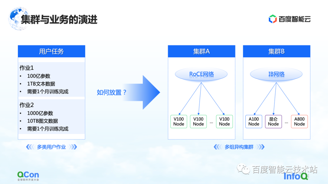
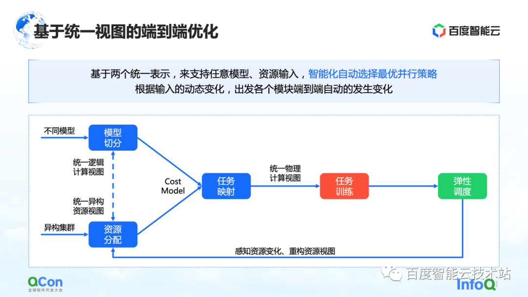
We have seen several methods now, one of which is end-to-end optimization based on a unified view: unify the entire model and heterogeneous resources on the view, and extend the Cost Model based on the unified view, which can support single-task and multi-job in Placement under heterogeneous resource clusters. Combined with the ability of elastic scheduling, it can better sense the changes of cluster resources.
All the capabilities mentioned above have been integrated into Baidu Baige's AI heterogeneous computing platform.
——END——
Recommended reading :
Talking about the application of graph algorithm in the activity scene in anti-cheating
Serverless: Flexible Scaling Practice Based on Personalized Service Portraits
Action decomposition method in image animation application
Performance Platform Data Acceleration Road
Editing AIGC Video Production Process Arrangement Practice
Baidu engineers talk about video understanding