Rec-Hub team study (1)

Task 4

ESMM (Ali cvr based on multi-task prediction training framework ESMM)

Due to business logic, different goals have explicit dependencies, such as exposure → click → conversion . The user must first click on the product in the product exposure interface before it is possible to purchase and convert. Ali proposed the ESMM (Entire Space Multi-Task Model) network, which explicitly models the joint training of tasks with dependencies. Although this model is a multi-task learning model, it essentially takes CVR as the main task, and introduces CTR and CTCVR as auxiliary tasks to solve the challenge of CVR estimation.

background and motivation

There are two main problems in the traditional CVR estimation problem: sample selection bias and sparse data . The white background in the figure below is exposure data, the gray background is click behavior data, and the black background is purchase behavior data. The training samples used for traditional CVR estimation are only gray and black data.

 

This causes two problems:

• Sample selection bias (SSB): As shown in the figure, the set of positive and negative samples of the CVR model = {negative samples that are not converted after clicking + positive samples that are converted after clicking}, but the online prediction is once the sample For exposure, it is necessary to predict CVR and CTR for sorting, sample set = {exposed samples}. The constructed training sample set is equivalent to sampling from a distribution that is inconsistent with the real distribution, which to some extent violates the assumption that training data and test data are independent and identically distributed in machine learning.
• Training data is sparse (data sparsity, DS): Click samples only account for a small part of the entire exposure samples, and conversion samples only account for a small part of the click samples. If only the post-click data is used to train the CVR model, the available samples will be extremely sparse.

solution

Alimama's team proposed ESMM, drawing on the idea of ​​multi-task learning, introducing two auxiliary tasks CTR and CTCVR (clicked and then converted), and eliminating the above two problems at the same time.

The three prediction tasks are as follows:

• pCTR：p(click=1 | impression)；
• pCVR: p(conversion=1 | click=1,impression)；
• pCTCVR: p(conversion=1, click=1 | impression) = p(click=1 | impression) * p(conversion=1 | click=1, impression)；

Note: Only when the labels of CTR and CVR are both 1 at the same time, the label of CTCVR is positive sample 1. If there is a sample with CTR=0 and CVR=1, it is an illegal sample and needs to be deleted. pCTCVR refers to the probability that the user will purchase if the user has already clicked; pCVR refers to the probability that the user will purchase if the user clicks.

The relationship between the three tasks is:

 Where x represents impressions, y represents clicks, and z represents conversions. For these three tasks, the model structure as shown in the figure is designed:

As shown in the figure, the main task and the auxiliary task share features. Different task output layers use different networks. The predicted value of cvr*ctr is used as the predicted value of the ctcvr task, and the loss function is constructed using the labels of ctcvr and ctr:

This architecture has two major characteristics, which respectively provide solutions to the above two problems:

• Helps the CVR model to model in the full sample space (i.e. exposure space X).

As can be seen from the formula, pCVR can be derived from pCTR and pCTCVR. In principle, it is equivalent to training two models separately to fit pCTR and pCTCVR, and then divide pCTCVR by pCTR to get the final fitting target pCVR. During the training process, the model only needs to predict pCTCVR and pCTR, and use the joint loss composed of the two additions to update the parameters. pCVR is only an intermediate variable. The data of pCTCVR and pCTR are extracted in the complete sample space, which means that pCVR is also modeled in the entire exposure sample space.

• Provides transfer learning of feature representation (embedding layer sharing). The two sub-networks of the CVR and CTR tasks share the embedding layer. The embedding layer of the network maps large-scale sparse input data to low-dimensional representation vectors. The parameters of this layer account for the vast majority of the entire network parameters and require a large number of training samples. to be fully learned. Since the training sample size of the CTR task is much larger than the training sample size of the CVR task, the feature representation sharing mechanism in the ESMM model can enable the CVR sub-task to learn from samples that only show but have no clicks, which can greatly facilitate training. Data sparsity problem.

After the model training is completed, the three indicators of cvr, ctr, and ctcvr can be predicted at the same time, and the online fusion can be performed according to actual needs or only the estimated value of cvr obtained by this model can be used.

Summary and Outlook

1. Can multiplication be replaced by division? That is, train the CTR and CTCVR models separately, and divide the two to obtain pCVR. The paper provides the results of the ablation experiment. The DIVISION model in the table has a significant improvement compared to the BASE model directly modeling CTCVRR and CVR, but is lower than ESMM. The reason is that pCTR is usually very small, and dividing by a small floating-point number can easily cause numerical instability.

   

2. Network structure optimization, Tower model replacement? The two towers are inconsistent? The subtask-independent Tower network in the original paper is a pure MLP model. In fact, the industry generally adopts more advanced models (such as DeepFM, DIN, etc.) during use. The two towers can also be set differently according to their own characteristics. model. This is also the advantage of the ESMM framework, the sub-network can be replaced arbitrarily, and it is very easy to integrate with other learning models.

3. Is there a better way than adding loss directly? The original paper directly adds the two losses, and can also introduce a dynamic weighted learning mechanism.

4. Longer sequence dependency modeling? Some business dependencies have more than exposure-click-conversion three layers, and the subsequent improved model proposes a deeper task dependency modeling.

   Ali's ESMM2: Before clicking to buy, users may also have behaviors such as adding to the shopping cart (Cart) and adding to the wish list (Wish).

​ Compared with directly learning click->buy (sparseness is about 2.6%), the target can be decomposed through the Action path, taking Cart as an example: click->cart (sparseness is 10%), cart->buy (sparseness is 10%) is 12%), by decomposing the path and establishing a multi-task learning model to solve the CVR model step by step to alleviate the sparsity problem, the model also introduces a feature sharing mechanism.

​ Meituan ’s AITM : In the credit card business, user conversion is usually a process of exposure -> click -> application -> verification card -> activation , with a 5-layer link.

 Meituan proposes an Adaptive Information Transfer Multi-task (**Adaptive Information Transfer Multi-task, AITM**) framework, which uses the Adaptive Information Transfer (AIT) module to implement sequence dependencies between users' multi-step transformations. modeling. The AIT module can adaptively learn what and how much information needs to be transferred in different transformation stages.

Summarize:

ESMM is the first to use user behavior sequence data to model in the complete sample space, and proposes to use the auxiliary tasks of learning CTR and CTCVR to learn CVR in a detour, avoiding the problems of sample selection bias and training data sparseness that traditional CVR models often encounter, and has achieved great success. significant effect.

MMOE was proposed by Google in 2018. The full name is Multi-gate Mixture-of-Experts. For multiple optimization tasks, multiple experts are introduced to make different decisions and combinations, and finally complete multi-objective prediction. What is solved is that in hard sharing, if the similarity of multiple tasks is not very strong, the underlying embedding learning will affect each other, and eventually they will not be able to learn the pain point.

This article first understands Hard-parameter sharing and existing problems, then leads to MMOE, sorts out the theoretical part, and finally refers to the simple reproduction of deepctr.

background and motivation

In the recommendation system, even in the same scene, there is often not only one business goal. In Youtube’s video recommendation, the recommendation sorting task not only needs to consider the user’s click-through rate and completion rate, but also some satisfaction indicators, such as whether the video is liked or not, and the user’s rating of the video after watching; In streaming product recommendations, click-through rate and conversion rate need to be considered; while in some content scenarios, indicators such as click and interaction, attention, and dwell time need to be considered.

In the model, if a network is used to complete multiple tasks at the same time, such a network model can be called a multi-task model. This model can learn the commonality and difference between different tasks, and can improve the quality and efficiency of modeling. The design paradigms of common multitasking models can be roughly divided into three categories:

• Hard parameter sharing method: This is a very classic method. The bottom layer is a shared hidden layer, which learns the common patterns of each task, and the upper layer uses some specific fully connected layers to learn specific task patterns.

  

  This method is also currently used, such as Meituan’s Guess You Like, Zhihu’s recommended Ranking, etc. The biggest advantage of this method is that the more tasks there are, the less likely it is to overfit a single task, that is, it can reduce the overfitting between tasks. Fitting risk. But the disadvantage is also very obvious, that is, it is difficult for the underlying mandatory shared layers to learn effective expressions suitable for all tasks. **Especially when there are conflicts between tasks**. The experimental conclusion is given in MMOE. When the correlation between the two tasks is not so good (such as the click-through rate and interaction in sorting, click and stay time), this result will suffer from training difficulties. After all, the bottom layer of all tasks is used. same set of parameters.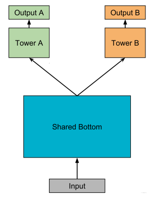

• soft parameter sharing: If hard ones don’t work, then use soft ones. The results corresponding to this paradigm will MOE->MMOE->PLEwait. That is, the bottom layer does not use a shared bottom, but has multiple towers, called multiple experts, and then there is often a gating network that assigns different weights to different towers during multi-task learning, so for different Tasks can allow the use of different combinations of experts in the bottom layer to make predictions. Compared with all the tasks above sharing the bottom layer, this method is more flexible

• Task sequence dependency modeling: This is suitable for certain sequence dependencies between different tasks. For example, ctr and cvr in the e-commerce scene, the behavior of cvr will only happen after clicking. Therefore, if this dependency can be utilized, it can solve the problem of sample selection bias (SSB) and data sparsity (DS) in task estimation.

  • 样本选择偏差: 后一阶段的模型基于上一阶段采样后的样本子集训练，但最终在全样本空间进行推理，带来严重泛化性问题Copy to clipboardErrorCopied

  • Sparse samples: The model training samples in the latter stage are much smaller than the tasks in the previous stage

    
    ESSM is a relatively general method for modeling task sequence dependencies. In addition, Ali's DBMTL, ESSM2 and other works all belong to this paradigm. This paradigm may be sorted out later, so I won’t repeat it in this article.

Through the above description, you can generally have an understanding of several common modeling paradigms in multi-task models, and then you also know some problems in hard parameter sharing, that is, you cannot balance the goals and tasks of specific tasks well. Conflict relationship. And this is one of the motivations proposed by the MMOE model. Then the key below is how does the MMOE model model the relationship between tasks, and how can a specific task and task relationship be kept in balance?

Multi-Task

• Scenario: Refinement (multi-task learning)

• Model: ESMM, MMOE

• Data: Ali-CCP dataset

• learning target

  • Learn to use torch-rechub to train an ESMM model
  • Learn to train an MMOE model based on torch-rechub

• learning materials:

  • Introduction to Multitasking Models: FunRec

  • Ali-CCP dataset official website: Dataset-Alibaba Cloud Tianchi

• Note: The hyperparameters in the model part of this tutorial have not been tuned. Friends are welcome to participate in parameter tuning and evaluation on the full amount of data after finishing the tutorial

#使用pandas加载数据
import pandas as pd
data_path = '' #数据存放文件夹
df_train = pd.read_csv(data_path + 'ali_ccp_train_sample.csv') #加载训练集
df_val = pd.read_csv(data_path + 'ali_ccp_val_sample.csv') #加载验证集
df_test = pd.read_csv(data_path + 'ali_ccp_test_sample.csv') #加载测试集
print("train : val : test = %d %d %d" % (len(df_train), len(df_val), len(df_test)))
#查看数据，其中'click'、'purchase'为标签列，'D'开头为dense特征列，其余为sparse特征，各特征列的含义参考官网描述
print(df_train.head(5)) 

Use torch-rechub to train the ESMM model

data preprocessing

In the data preprocessing process usually need:

• Lable Encode sparse classification features
• Bucket or normalize numerical features

Since the sampled data and full data in this tutorial have been preprocessed, the loaded data set can be used directly.

The task of this multi-task model is to predict clicks and purchase tags, which are typical CTR and CVR prediction tasks in recommendation systems.

train_idx, val_idx = df_train.shape[0], df_train.shape[0] + df_val.shape[0]
data = pd.concat([df_train, df_val, df_test], axis=0)
#task 1 (as cvr): main task, purchase prediction
#task 2(as ctr): auxiliary task, click prediction
data.rename(columns={'purchase': 'cvr_label', 'click': 'ctr_label'}, inplace=True)
data["ctcvr_label"] = data['cvr_label'] * data['ctr_label']

define model

To define a model, you need to specify the model structure parameters. For which parameters are required, you can check the definition part of the corresponding model. For ESMM, the main parameters are as follows:

• user_features refers to the features on the user side, and can only be passed in the sparse type (in the paper, the sum_pooling operation needs to be performed on the features on the user and item sides respectively)
• item_features refers to the features on the item side, and only the sparse type can be passed in
• cvr_params specifies the parameters of the MLP layer in CVR Tower
• ctr_params specifies the parameters of the MLP layer in CTR Tower

from torch_rechub.models.multi_task import ESMM
from torch_rechub.basic.features import DenseFeature, SparseFeature

col_names = data.columns.values.tolist()
dense_cols = ['D109_14', 'D110_14', 'D127_14', 'D150_14', 'D508', 'D509', 'D702', 'D853']
sparse_cols = [col for col in col_names if col not in dense_cols and col not in ['cvr_label', 'ctr_label']]
print("sparse cols:%d dense cols:%d" % (len(sparse_cols), len(dense_cols)))
label_cols = ['cvr_label', 'ctr_label', "ctcvr_label"]  #the order of 3 labels must fixed as this
used_cols = sparse_cols #ESMM only for sparse features in origin paper
item_cols = ['129', '205', '206', '207', '210', '216']  #assumption features split for user and item
user_cols = [col for col in used_cols if col not in item_cols]
user_features = [SparseFeature(col, data[col].max() + 1, embed_dim=16) for col in user_cols]
item_features = [SparseFeature(col, data[col].max() + 1, embed_dim=16) for col in item_cols]

model = ESMM(user_features, item_features, cvr_params={"dims": [16, 8]}, ctr_params={"dims": [16, 8]})

build dataloader

Building a dataloader is usually done by

1. Build an input dictionary (the key of the dictionary is the feature name used when defining the model, and the value is the data of the corresponding feature)
2. Build the corresponding dataset and dataloader through the dictionary

from torch_rechub.utils.data import DataGenerator

x_train, y_train = {name: data[name].values[:train_idx] for name in used_cols}, data[label_cols].values[:train_idx]
x_val, y_val = {name: data[name].values[train_idx:val_idx] for name in used_cols}, data[label_cols].values[train_idx:val_idx]
x_test, y_test = {name: data[name].values[val_idx:] for name in used_cols}, data[label_cols].values[val_idx:]
dg = DataGenerator(x_train, y_train)
train_dataloader, val_dataloader, test_dataloader = dg.generate_dataloader(x_val=x_val, y_val=y_val, 
                                      x_test=x_test, y_test=y_test, batch_size=1024)

Train the model and test

• The training model is carried out through the corresponding trainer. For the multi-task MTLTrainer, it is necessary to set the type of task, the hyperparameters of the optimizer, and the optimization strategy.

• Test on the test set after model training

import torch
import os
from torch_rechub.trainers import MTLTrainer
device = 'cuda' if torch.cuda.is_available() else 'cpu'
learning_rate = 1e-3
epoch = 1 #10
weight_decay = 1e-5
save_dir = '../examples/ranking/data/ali-ccp/saved'
if not os.path.exists(save_dir):
    os.makedirs(save_dir)
task_types = ["classification", "classification"] #CTR与CVR均为二分类任务
mtl_trainer = MTLTrainer(model, task_types=task_types, 
              optimizer_params={"lr": learning_rate, "weight_decay": weight_decay}, 
              n_epoch=epoch, earlystop_patience=1, device=device, model_path=save_dir)
mtl_trainer.fit(train_dataloader, val_dataloader)
auc = mtl_trainer.evaluate(mtl_trainer.model, test_dataloader)
print(f'test auc: {auc}')

Theory and paper details of the MMOE model

The MMOE model structure diagram is as follows.

This is actually a process of evolution. First of all, hard parameter sharing does not need to be described too much. The following mainly looks at the MOE model and the MMOE model.

mixed expert model

We know that this shared model structure will suffer from conflicts between tasks and may not converge well, so that common patterns between tasks cannot be learned. This structure can also be seen as sharing an expert for multiple tasks.

Putting aside the task relationship first, we found that an expert has limited expressive ability in multi-task learning, so we tried to introduce multiple experts, which slowly evolved a mixed expert model. The formula is expressed as follows:

Here yy represents the aggregated output of multiple experts, and then this thing has to go through a specific task tower to get the output of a specific task. A gating network mechanism is also added here, which is an attention network to learn the importance weight of each expert\sum_{i=1}^{n} g(x)_{i}=1∑i=1n​ g(x)i​=1. f_i(x)fi​(x) is the output of each expert, and g(x)_ig(x)i​is the weight corresponding to each expert. Although I feel that this thing is nothing more than introducing several fully connected networks on the basis of a single expert, and then weighting these fully connected networks, but in my opinion, there are at least several powerful ideas in it:

1. The idea of ​​model integration: This thing is very similar to the idea of ​​bagging, that is, to train multiple models to make decisions. The effectiveness of this decision is obviously more reliable than that of a single model, no matter in terms of generalization ability, expression ability, and learning ability. , should both be stronger than a model
2. Attention idea: In order to increase flexibility, importance weights are also learned for different models, which may take into account that different models learn different modes in the common mode of learning tasks, so when aggregation, it is obviously not possible to follow the same The importance is aggregated, so the weights are learned for each expert, and the decision-making status of different experts is different by default. This idea is now very common.
3. Multi-head mechanism: From another perspective, multiple experts actually represent multiple different heads, and different heads represent different nonlinear spaces. The reason why the expression ability is enhanced is because the input features are mapped to different to learn the common pattern between tasks in the space. It can be understood as capturing the common feature patterns between tasks from multiple perspectives.

MOE uses multiple mixed experts to increase various expressive capabilities. However, a gate is not very flexible, because all these tasks can only select a group of expert combinations, that is, this expert combination is on multiple tasks. The results of the comprehensive measurement are not targeted anymore. If these tasks are relatively similar, it means that this group of experts can indeed deal with these multiple tasks and learn the commonality of multiple similar tasks. But if there is a big difference between tasks, this single-gate control method will not work, because at this time the feature patterns learned by multiple experts at the bottom may differ greatly. After all, the tasks are different, and the single-gate control mechanism When choosing a combination of experts, we must choose those experts who are beneficial to most tasks, but for some special tasks, they may learn a mess.

Therefore, the gap in this method is obvious. In this way, it is more understandable why the expert mixture model of multi-gate control is proposed.

MMOE structure

The charm of Multi-gate Mixture-of-Experts (MMOE) is that on the basis of OMOE, a gating network is involved for each task, so that for each specific task, there can be a set of corresponding expert combinations to Make predictions. When it is more critical, the amount of parameters will not increase too much. The formula is as follows: kk here represents the number of tasks. Each gating network is an attention network:

 

 

Represents the weight matrix, n is the number of experts, and d is the dimension of the feature.

 

The above formula does not need too much explanation here.

This transformation seems very simple, just adding a few extra gated networks on OMOE, but it has a leverage-like effect. I will share my understanding here.

• First of all, with regard to the OMOE problem just analyzed, a single gating will limit the selection of expert combinations. At this time, if multiple tasks conflict, this structure cannot make a good trade-off. But MMOE is different. MMOE has a separate gate selection expert combination for each task, so even if the task conflicts, it can be adjusted according to different gates, and an expert combination that is helpful for the current task can be selected. Therefore, I think single-gate control achieves the decoupling of expert selection for all tasks , while multi-gate control achieves decoupling of expert combination selection for each task .
• The multi-gating mechanism is now able to model the relationship between tasks. If each task conflicts, then multi-gated help is available at this time. At this time, let each task have an exclusive expert. If the tasks can be clustered into several similar categories, then the corresponding differences between these categories should be The combination of experts, then the gating mechanism can also be selected. If all tasks are similar, the weights learned by these gated networks will also be similar, so this mechanism unifies the irrelevance, partial correlation and full correlation of tasks.
• Flexible parameter sharing. This can be compared with the hard mode or the model that is modeled separately for each task. For the hard mode, all tasks share the underlying parameters, and each task is modeled separately, so all tasks have a separate set of parameters. It can be regarded as the two extremes of sharing and non-sharing. For the extreme of sharing, fear of task conflicts, and for the extreme of not sharing at all, the advantages of transfer learning cannot be used, and the models cannot share information with each other. Complementary, easy Suffering from the predicament of overfitting, it will also increase the amount of calculations and parameters. MMOE is in the middle of the two, taking into account that if there are similar tasks, then the parameters will be shared, the modes will be shared, and complement each other. If there are no similar tasks, then learn independently without affecting each other. These two extremes were unified again.
• It can converge quickly during training, because similar tasks will contribute to the training of specific expert combinations, so one round of epoch is equivalent to multiple rounds of epoch in single task training.

OK, the story of the MMOE has been sorted out here. The model structure itself is not very complicated, which is very in line with the principle of "simplification from the road", simple and practical.

So, why is multi-task learning effective? Here is a good answer to see:

The reason why multi-task learning is effective is the introduction of inductive bias, two effects:

• Mutual promotion: The relationship between multi-task models can be regarded as mutual prior knowledge, also known as inductive transfer. With prior assumptions about the model, the effect of the model can be better improved. Solving data sparsity is actually a feature of transfer learning itself, and it will also be reflected in multi-task learning
• Generalization: Different models learn different representations. It is possible that model A learns what model B has not learned well, and model B also has its own characteristics, which is likely to be poor in A. This will improve the robustness of the model. stronger

Use torch-rechub to train the MMOE model

The process of training the MMOE model is very similar to the ESMM model

It should be noted that the MMOE model supports both dense and sparse features as input, as well as a mixture of classification and regression tasks

from torch_rechub.models.multi_task import MMOE
# 定义模型
used_cols = sparse_cols + dense_cols
features = [SparseFeature(col, data[col].max()+1, embed_dim=4)for col in sparse_cols] \
                   + [DenseFeature(col) for col in dense_cols]
model = MMOE(features, task_types, 8, expert_params={"dims": [16]}, tower_params_list=[{"dims": [8]}, {"dims": [8]}])
#构建dataloader
label_cols = ['cvr_label', 'ctr_label']
x_train, y_train = {name: data[name].values[:train_idx] for name in used_cols}, data[label_cols].values[:train_idx]
x_val, y_val = {name: data[name].values[train_idx:val_idx] for name in used_cols}, data[label_cols].values[train_idx:val_idx]
x_test, y_test = {name: data[name].values[val_idx:] for name in used_cols}, data[label_cols].values[val_idx:]
dg = DataGenerator(x_train, y_train)
train_dataloader, val_dataloader, test_dataloader = dg.generate_dataloader(x_val=x_val, y_val=y_val, 
                                      x_test=x_test, y_test=y_test, batch_size=1024)
#训练模型及评估
mtl_trainer = MTLTrainer(model, task_types=task_types, optimizer_params={"lr": learning_rate, "weight_decay": weight_decay}, n_epoch=epoch, earlystop_patience=30, device=device, model_path=save_dir)
mtl_trainer.fit(train_dataloader, val_dataloader)
auc = mtl_trainer.evaluate(mtl_trainer.model, test_dataloader)

 

Task3

Twin Towers Recall Model

The twin-tower model is a very classic model in the field of recommendation, and it will be the first choice whether it is in the recall or rough sorting stage. This is mainly due to the two-tower model structure, which enables the low-latency requirements to be met during online estimation. But it is also because of the problem of its model structure that it is impossible to consider the feature intersection between user and item characteristics, which affects the final effect of the model. Therefore, many works try to adjust the structure of the classic two-tower model, while maintaining low latency in online estimation. , to ensure effective information crossing between the two sides of the twin towers. The following is an introduction to the classic twin-tower model and some improved versions.

Classic twin tower model

DSSM (Deep Structured Semantic Model) is a work proposed by Microsoft Research in CIKM in 2013. This model is mainly used to solve the semantic similarity task in the NLP field. It uses a deep neural network to represent text as a low-dimensional vector. To improve the matching of documents and queries in search scenarios. The principle of the DSSM model is mainly: through the log data of query and doc in the user search behavior, the query and doc are mapped to the semantic space of the common dimension through the deep learning network, and by maximizing the cosine similarity between the query and doc semantic vectors Degree, so as to train the implicit semantic model, that is, the embedding of the query side feature and the embedding of the doc side feature, and then obtain the low-dimensional semantic vector expression sentence embedding of the sentence, and predict the semantic similarity between two sentences. The model structure looks like this:

In the recommendation system, the most critical issue is how to match users and items well. Therefore, the DSSM model in the recommendation system is to build independent sub-network tower structures for users and items, and use the relationship between users and items. Expose or click on the date for training, and finally get the embedding on the user side and the embedding on the item side. Therefore, in the recommendation system, the common model structure is as follows

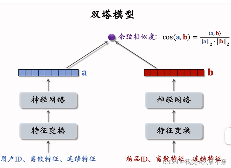
 From the perspective of the model structure, it mainly includes two parts: the user side tower and the item side tower, and each tower is a DNN structure. Through the feature input on both sides, through the DNN module to the embedding of user and item, and then calculate the similarity between the two (commonly used inner product or cosine value, the connection and difference between these two methods will be described below), so for user The embedding dimension finally obtained on both sides of the item needs to be consistent, that is, the number of hidden units in the last fully connected layer is the same.

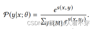
In the recall model, this retrieval behavior is treated as a multi-class classification problem, similar to the YouTubeDNN model. Treat all items in the material library as a category, so the loss function needs to calculate the probability value of each category:

 

 The above is the classic two-tower model in the recommendation system. The reason why it is very common in practical applications is that in the scenario of recalling a large amount of candidate data, the speed is very fast, and the effect is not extremely good, but generally speaking, the effect is enough. up . The reason why the two-tower model is fast in service is because the model structure is simple (there is no feature intersection on both sides), but this also brings problems. The structure of the two-tower model cannot consider the interactive information between the features on both sides . To a certain extent, part of the accuracy of the model is sacrificed . For example, in the fine-tuning model, the features from the user side and the item side can perform fine-grained feature interaction in the first NLP layer, while for the two-tower model, the features from the user side and the item side will only be in the final layer. This happens when the product is calculated, which causes a lot of useful information to be blurred by other features when it passes through the DNN structure. Therefore, the twin-tower structure inherently has such problems due to its structural problems. Let's take a look at the solution ideas of the existing models for this problem.

SENet Twin Towers Model

SENet was proposed by Momenta in 2017, when it was a new network structure applied to image processing. Later, Mr. Zhang Junlin introduced SENet into the fine-tuning model FiBiNET . Its function is to discard a large number of long-tail low-frequency features, weaken the negative impact of unreliable low-frequency feature embedding, and strengthen the important role of high-frequency features. So what exactly is the SENet structure, and why can it play a role in feature screening?

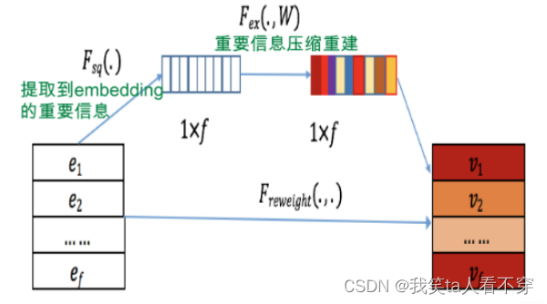
It can be seen from the figure above that SENET is mainly divided into three steps Squeeze, Excitation, Re-weight:

• Squeeze stage: We perform data compression and information summary on the Embedding vector of each feature, that is, calculate the mean value in the Embedding dimension:

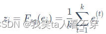
 Where k represents the dimension of Embedding, and the Squeeze stage is to convert the Squeeze of each feature into a single value.

 

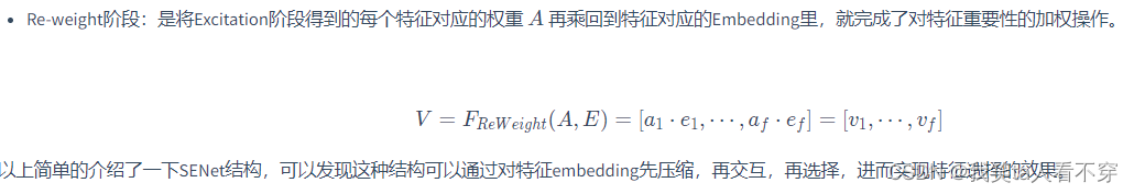
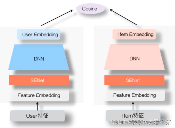
As can be seen from the above figure, specifically, a SENet module is added to the feature input part of the user tower and the Item side tower in the twin towers, and the importance of these features is dynamically learned through the SENet network, and noise or invalidity is suppressed through small weights. Low-frequency features, the purpose of amplifying the influence of important features through large weights.

Why is the SENet twin-tower model effective? Mr. Zhang Junlin’s explanation is: The problem with the two-tower model is that the interaction between User-side features and Item-side features is too late. Interaction at a high level will cause the loss of detailed information, that is, specific feature information, and affect the effect of feature crossover on both sides. The SENet module filters features at the bottom layer, so that even if many invalid low-frequency features are filtered out, more useful information is retained at the top layer of the twin towers, making the crossover effect on both sides very good; at the same time, due to SENet The module selects more important information, which enhances the ability of DNN twin towers in terms of interactive expression between User side and Item side features.

Therefore, the SENet twin-tower model mainly improves the effectiveness of feature crossover on both sides from the perspective of feature selection, reduces the interference of noise on effective information, and then improves the effect of the twin-tower model. In addition, in addition to this method, the information interaction between the two sides can also be enhanced by adding channels. That is to say, not only a DNN structure is used on both sides of user and item, but the self-feature intersection of user and item can be modeled through different structures (such as FM, DCN, etc.), as shown in the following figure:

 In this way, multiple embeddings will be obtained for the user and item sides, similar to the concept of multiple interests. By obtaining the embeddings of multiple users and items, and then calculating the cosine values ​​separately and adding them together (the Embedding dimensions on both sides need to be aligned), this increases the information interaction on both sides of the twin towers. And this method has been tried in Tencent, and the "parallel" twin towers they proposed are based on this idea, and those who are interested can find out.

Multi-objective twin-tower model

Nowadays, multi-task learning is also very common in actual application scenarios, mainly because the business in actual scenarios is complex, and there are often many measurement indicators, such as clicks, comments, favorites, attention, forwarding, etc. In multi-task learning, a unique tower is often used for different tasks, and then the loss of different tasks is optimized. So how to build a multi-task learning framework for the twin tower model?

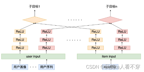
 As shown in the figure above, a user embedding and item embedding are obtained for each task through multiple channels (DNN structure) on the user side and item side, and then the similarity between user and item is calculated for different targets, and each target is calculated The final optimization objective can be the sum of multiple task losses, or use dynamic loss weights in multi-task learning.

This model structure can jointly model multiple targets. Through the structure of multi-task learning, on the one hand, it can use the information sharing between different tasks to provide some sparse features with migration information in other tasks. When recalling, one model is directly used to obtain multiple target predictions, which solves the problem of difficult maintenance of multiple models. That is to say, multiple indicators can be obtained at the same time through this model online. For example, in video scenes, a model can directly obtain the predicted values ​​of targets such as likes, comments, and retweets, and then use these values ​​to calculate scores to obtain the final result. Top-K recall results.

Twin Towers Model Details: Reference: FunRec

Combat practice

Torch-Rechub Tutorial：Matching

• Scenario: Recall
• Models: DSSM, YouTubeDNN

• Data: MovieLens-1M

• This tutorial covers the following:

  1. Dataset training a DSSM recall model on the MovieLens-1M dataset
  2. Dataset Training a YouTubeDNN Recall Model on the MovieLens-1M Dataset

• Before reading this tutorial, I hope you have a preliminary understanding of YouTubeDNN and DSSM, and a general understanding of how data flows in the model, otherwise you may be confused when you directly code. Model Introduction: YouTubeDNN  DSSM

• This tutorial is a more detailed explanation of examples/matching/run_ml_dssm.pythe examples/matching/run_ml_youtube_dnn.pytwo files, and the code is basically consistent with the two files.
• This framework is still under development and may still have some bugs. If you find that the indicator is significantly higher than the current one after the recovery, welcome to communicate with us.

import torch
import pandas as pd
import numpy as np
import os
pd.set_option('display.max_rows',500)
pd.set_option('display.max_columns',500)
pd.set_option('display.width',1000)
torch.manual_seed(2022)


file_path = 'ml-1m_sample.csv'
data = pd.read_csv(file_path)
print(data.head())

feature preprocessing

In this DSSM model, we use two types of features, namely sparse features (SparseFeature) and sequence features (SequenceFeature).

• For sparse features, it is a discrete and limited value (such as user ID, which is generally converted into a continuous integer value by LabelEncoding operation first), and the model inputs it to the Embedding layer and outputs an Embedding vector.

• For sequence features, each sample is a List[SparseFeature] (usually viewing history, search history, etc.). For this feature, by default, the Embedding is averaged for each element, and an Embedding vector is output. In addition, in addition to the average, there are splicing, the most value, etc., which can be specified in the pooling parameter.

• The framework also supports dense features (DenseFeature), that is, a continuous feature value (such as probability), which generally needs to be normalized. But it is not used in this example.

The above three types of characteristics are defined intorch_rechub/basic/features.py

# 处理genres特征，取出其第一个作为标签
data["cate_id"] = data["genres"].apply(lambda x: x.split("|")[0])

# 指定用户列和物品列的名字、离散和稠密特征，适配框架的接口
user_col, item_col = "user_id", "movie_id"
sparse_features = ['user_id', 'movie_id', 'gender', 'age', 'occupation', 'zip', "cate_id"]
dense_features = []


save_dir = 'saved/'
if not os.path.exists(save_dir):
    os.makedirs(save_dir)
# 对SparseFeature进行LabelEncoding
from sklearn.preprocessing import LabelEncoder
print(data[sparse_features].head())
feature_max_idx = {}
for feature in sparse_features:
    lbe = LabelEncoder()
    data[feature] = lbe.fit_transform(data[feature]) + 1
    feature_max_idx[feature] = data[feature].max() + 1
    if feature == user_col:
        user_map = {encode_id + 1: raw_id for encode_id, raw_id in enumerate(lbe.classes_)}  #encode user id: raw user id
    if feature == item_col:
        item_map = {encode_id + 1: raw_id for encode_id, raw_id in enumerate(lbe.classes_)}  #encode item id: raw item id
np.save(save_dir+"raw_id_maps.npy", (user_map, item_map))  # evaluation时会用到
print('LabelEncoding后：')
print(data[sparse_features].head())

User Tower and Item Tower

In DSSM, it is divided into user tower and item tower, and the output of each tower is obtained by MLP (multi-layer perceptron) after splicing user/item features. Let's define the characteristics of the item tower and the user tower:

# 定义两个塔对应哪些特征
user_cols = ["user_id", "gender", "age", "occupation", "zip"]
item_cols = ['movie_id', "cate_id"]

# 从data中取出相应的数据
user_profile = data[user_cols].drop_duplicates('user_id')
item_profile = data[item_cols].drop_duplicates('movie_id')
print(user_profile.head())
print(item_profile.head())

Processing of sequence features

The sequence feature in this data set is the viewing history, which is generated according to the timestamp, and is specifically implemented in the generate_seq_feature_matchfunction. The meaning of the parameters is as follows:

• modeIndicates the training method of the sample (0 - point wise, 1 - pair wise, 2 - list wise)
• neg_ratioIndicates the number of negative samples corresponding to each positive sample,
• min_itemLimit the minimum sample size for each user. If the value is less than this value, it will be discarded and treated as a cold start user (the cold start processing has not been added to the framework, so it is directly discarded here)
• sample_methodIndicates the negative sampling method.

modeA little note about the parameters : In the process of model implementation, the framework only considers the training method of the samples proposed in the paper, and errors may be reported in other ways. For example: DSSM adopts the point wise method, that is mode=0, if it is passed modein, it is not guaranteed to run correctly, but the corresponding training method in the paper can guarantee correct operation.

from torch_rechub.utils.match import generate_seq_feature_match, gen_model_input
df_train, df_test = generate_seq_feature_match(data,
                                               user_col,
                                               item_col,
                                               time_col="timestamp",
                                               item_attribute_cols=[],
                                               sample_method=1,
                                               mode=0,
                                               neg_ratio=3,
                                               min_item=0)
print(df_train.head())
x_train = gen_model_input(df_train, user_profile, user_col, item_profile, item_col, seq_max_len=50)
y_train = x_train["label"]
x_test = gen_model_input(df_test, user_profile, user_col, item_profile, item_col, seq_max_len=50)
y_test = x_test["label"]
print({k: v[:3] for k, v in x_train.items()})



#定义特征类型

from torch_rechub.basic.features import SparseFeature, SequenceFeature
user_features = [
    SparseFeature(feature_name, vocab_size=feature_max_idx[feature_name], embed_dim=16) for feature_name in user_cols
]
user_features += [
    SequenceFeature("hist_movie_id",
                    vocab_size=feature_max_idx["movie_id"],
                    embed_dim=16,
                    pooling="mean",
                    shared_with="movie_id")
]

item_features = [
    SparseFeature(feature_name, vocab_size=feature_max_idx[feature_name], embed_dim=16) for feature_name in item_cols
]
print(user_features)
print(item_features)

# 将dataframe转为dict
from torch_rechub.utils.data import df_to_dict
all_item = df_to_dict(item_profile)
test_user = x_test
print({k: v[:3] for k, v in all_item.items()})
print({k: v[0] for k, v in test_user.items()})

training model

• Generate Dataloader for training (train_dl) and Dataloader for testing (test_dl, item_dl) based on the previous x_train dictionary and y_train data.

• Define a two-tower DSSM model, user_featureswhich represents the characteristics of the user_paramsuser tower, and represents the dimensions and activation functions of each layer of the MLP of the user tower. (Note: In this example, the selection of the activation function has a great influence on the final result. Do not modify the parameters of the activation function during debugging)

• Define a recall trainer MatchTrainer for model training.

from torch_rechub.models.matching import DSSM
from torch_rechub.trainers import MatchTrainer
from torch_rechub.utils.data import MatchDataGenerator
# 根据之前处理的数据拿到Dataloader
dg = MatchDataGenerator(x=x_train, y=y_train)
train_dl, test_dl, item_dl = dg.generate_dataloader(test_user, all_item, batch_size=256)

# 定义模型
model = DSSM(user_features,
             item_features,
             temperature=0.02,
             user_params={
                 "dims": [256, 128, 64],
                 "activation": 'prelu',  # important!!
             },
             item_params={
                 "dims": [256, 128, 64],
                 "activation": 'prelu',  # important!!
             })

# 模型训练器
trainer = MatchTrainer(model,
                       mode=0,  # 同上面的mode，需保持一致
                       optimizer_params={
                           "lr": 1e-4,
                           "weight_decay": 1e-6
                       },
                       n_epoch=1,
                       device='cpu',
                       model_path=save_dir)

# 开始训练
trainer.fit(train_dl)

Vectorized recall evaluation

• Use the trainer to obtain the embedding of each user in the test set and the embedding set of all items in the data set
• Use annoy to build an item embedding index, and perform ANN (Approximate Nearest Neighbors) for each user vector to recall K items
• View the topk evaluation indicators, generally look at recall, precision, hit

import collections
import numpy as np
import pandas as pd
from torch_rechub.utils.match import Annoy
from torch_rechub.basic.metric import topk_metrics

def match_evaluation(user_embedding, item_embedding, test_user, all_item, user_col='user_id', item_col='movie_id',
                     raw_id_maps="./raw_id_maps.npy", topk=10):
    print("evaluate embedding matching on test data")
    annoy = Annoy(n_trees=10)
    annoy.fit(item_embedding)

    #for each user of test dataset, get ann search topk result
    print("matching for topk")
    user_map, item_map = np.load(raw_id_maps, allow_pickle=True)
    match_res = collections.defaultdict(dict)  # user id -> predicted item ids
    for user_id, user_emb in zip(test_user[user_col], user_embedding):
        items_idx, items_scores = annoy.query(v=user_emb, n=topk)  #the index of topk match items
        match_res[user_map[user_id]] = np.vectorize(item_map.get)(all_item[item_col][items_idx])

    #get ground truth
    print("generate ground truth")

    data = pd.DataFrame({user_col: test_user[user_col], item_col: test_user[item_col]})
    data[user_col] = data[user_col].map(user_map)
    data[item_col] = data[item_col].map(item_map)
    user_pos_item = data.groupby(user_col).agg(list).reset_index()
    ground_truth = dict(zip(user_pos_item[user_col], user_pos_item[item_col]))  # user id -> ground truth

    print("compute topk metrics")
    out = topk_metrics(y_true=ground_truth, y_pred=match_res, topKs=[topk])
    return out

user_embedding = trainer.inference_embedding(model=model, mode="user", data_loader=test_dl, model_path=save_dir)
item_embedding = trainer.inference_embedding(model=model, mode="item", data_loader=item_dl, model_path=save_dir)
match_evaluation(user_embedding, item_embedding, test_user, all_item, topk=10, raw_id_maps=save_dir+"raw_id_maps.npy")

YouTubeNN recall

The YouTubeDNN model is an article in 2016. Although it is a bit far away from now, this article is undoubtedly a model of industry papers. It is completely thinking about how to make a recommendation system from the perspective of the industry, and YouTube is everywhere. The valuable experience left by the engineer, because I have used this model in the past two days, I just revisited this article today, so let’s take this opportunity to sort it out. Teacher Wang Zhe called this article "Shenwen" ", it can be seen that it is unusual.

After reading it today, I felt the biggest feeling. First of all, I analyzed the entire recommendation system from an engineering point of view, and talked about the two most important modules in the recommendation system: recall and sorting. This paper is very friendly to beginners. Before It is impossible to see such a comprehensive system in the thesis model, and there is always a feeling of being in control, unable to see the overall situation, and easy to fall into the trap. Secondly, this article gives a lot of engineering experience in optimizing the recommendation system. Whether it is recall or sorting, there are many routines or tricks, such as "example age", "negative sampling" and "asymmetrical" in terms of recall. Consumption, prevent leakage", feature engineering in sorting, weighted logistic regression, etc. These things are still very practical so far, so this is also the strength of this article.

This article is still based on paper. First, analyze every detail in the paper. Of course, I also refer to articles written by other big guys. Several articles written by Mr. Wang Zhe are very good. I also put the link Below, it is recommended to take a look. Then there is how to use the YouTubeDNN model, the code reproduction part, because the time is relatively short, I will not reproduce it first, adjust the deepmatch package to run, and then conduct some experiments on the news recommendation data set, and try some of the papers. Method, here is mainly how to use the YouTubeDNN model of deepmatch, as well as my thoughts and thoughts throughout the experiment process, because the structure of this model is not very complicated in nature (three or four layers of fully connected networks), so I don’t Let's implement it again, some engineering experience or ideas, I think it is the essence of this article.

Introduction and the Funnel Paradigm for Recommender Systems

Introduction

This paper is an engineering paper (the previous DIN is also a paper that is partial to engineering practice), and its writing style is mainly based on practical applications. We know that YouTube is a global video website, so this article mainly describes the development of the YouTube video recommendation system. The basic structure and details, as well as various processing tricks.

In the Introduction section, the author first stated the three major challenges faced by the industrial YouTube video recommendation system:

1. Scale (scale): The number of videos is very large. Large-scale data requires distributed learning algorithms and efficient online service systems. This is reflected in the article when the recall model is trained offline. The idea of ​​​​negative sampling is adopted. Online When serving, hash mapping is used, and then neighbor retrieval is used to meet real-time requirements. I have sorted out the use of faiss package and annoy package before, if you are interested, you can take a look. In fact, on a higher level, the overall structure of our recommendation system is in the funnel paradigm, which is also to ensure real-time recommendations from large-scale scenarios.
2. Freshness: Videos on YouTube are dynamic. Users upload and access them in real time. At this time, the latest videos are often easy to attract users' attention. Users generally prefer to watch newer videos. Regardless of whether it is really related to users (this feeling is similar to news), at this time, the model needs to have the ability to model newly uploaded content and the latest behavior of users. In order for the model to learn that users have preferences for new videos, an "example age" is added to the strategy later as a reflection. The exploration in what we call "exploration and utilization" is actually the grasp of freshness.
3. Noise: Due to data sparsity and other invisible reasons, there is a lot of noise in the data. At this time, it is necessary to make this recommendation system robust. How to be robust? This involves recall and sorting. More practical factors need to be considered in recall, such as asymmetric consumption characteristics, high-active user factors, time factors, sequence factors, etc., and corresponding measures have been taken, while sorting should be more detailed Feature engineering, try to describe user interests and video features to optimize training goals, use weighted logistic regression, etc. The recall and sorting models both use a deep neural network, which has a stronger modeling ability through the mutual intersection of features. Compared with the previous MF (matrix decomposition), the modeling ability has greatly improved. These are all helpful to help reduce noise and make the recommendation results more accurate.

Therefore, from the perspective of the overall logic of the article, the details in the following are actually developed around the challenges. If you find the problems facing the current recommendation, you have to find a way to solve the problems, so the logic of this article is also very clear.

Knowing the challenges, let's take a look at the overall recommendation system architecture of YouTubeDNN.

The entire recommendation architecture diagram is as follows, which is a relatively primitive funnel structure:

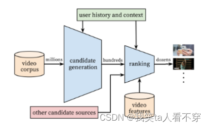
The reason why this article is well written is that it gives us a macro perspective on the recommendation system. This system is mainly composed of two parts: recall and sorting. The purpose of the recall is to quickly find items of potential interest to a small number of users from the massive item library based on some characteristics of users and hand them over to fine sorting. The emphasis is on speed. Fine sorting is mainly to incorporate more features and use complex models for personalization Recommended, emphatically accurate.

As for the specific description of these two parts, the paper also gives an explanation. Here I simply expand the mainstream method based on my current understanding:

recall side

The input of the recall side model is generally the user's click history, because we believe that these histories can better represent the user's interests, and there are also some demographic characteristics, such as gender, age, region, etc., which can be used as the recall side model. enter. The output of the final model is a set of candidate videos related to the user, and the order of magnitude is usually several hundred.
On the recall side, according to my understanding, there are generally two types of recall methods, one is policy rules, and the other is supervisory model + embedding. Among them, policy rules are often related to real scenarios, such as popularity, historical redirection, etc. , Different scenarios will have different recall methods, which belongs to "specificity" knowledge.
The following model + embedding idea is a "universal" method. I sorted out the current mainstream methods for embedding users and items in the above figure. These methods are roughly divided into several series, such as FM series (FM, FFM, etc.) , user behavior sequence, graph-based and knowledge graph series, classic twin-tower series, etc. These methods seem to be many and complicated, but in fact they are just embedding users or items in essence, but the angles of consideration are different. The YouTubeDNN recall model here is also a way here.

Finishing side

For each user on the recall side, hundreds of relatively relevant candidate videos are given, and the scale of millions is reduced to a few hundred. Of course, the feature information used on the recall side is limited, which cannot describe users and Video features. Therefore, on the fine layout side, the main purpose is to use more users, video features, and describe features more accurately. Select a few or a dozen from these hundreds and recommend them to users. When it comes to standards, there are generally three main points of effort: feature engineering, model design, and training methods. Almost all of these three focus articles are involved. Except for the mode design, which is a bit judging the situation, the handling of feature engineering and training methods is very beautiful, and the details will be sorted out later.
On the refinement side, the general development trend of this area is from ctr estimation to multi-objective, and in terms of model evolution, from manual feature engineering to feature engineering automation. There are mainly three blocks. CTR estimation is mainly divided into the traditional LR, FM family, and the DNN family with automatic feature crossing. Multi-objective optimization is currently the research status of many large companies, and it is a major development in the future. Trends, how to make the model learn "with ease" on each goal is a very challenging thing. After all, different goals may conflict with each other and affect each other, so the research hotspots here can be split into network structures. Evolution and loss design optimization, etc. In the evolution of the network structure, it can be subdivided again. Of course, almost every model or technology has a corresponding paper, and we can still learn these key technologies by reading the paper.

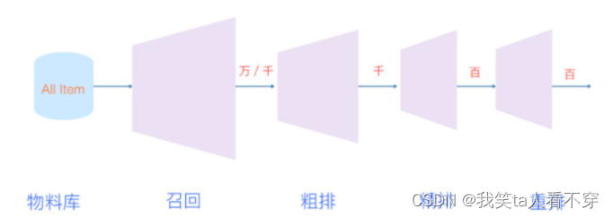
The two-stage method can ensure that we can make real-time recommendations from a large-scale video library, and can also ensure personalization and attract users. Of course, with the development of time, the amount of data may be very, very large. At this time, the scale of recall results cannot be processed by fine sorting, so now generally a rough sorting is added as a transition between recall and fine sorting, and As the scene becomes more and more complex, the result of fine sorting is not directly given to the user, but will be processed after adding a rearrangement. This paper actually briefly mentions this idea, in sorting That piece will be sorted out. So today's funnel has also become longer.

 The paper also mentions the evaluation of the model. When evaluating offline, it mainly uses some commonly used evaluation indicators (precision rate, recall rate, sorting loss or auc), but in the end it depends on the effectiveness of the algorithm and model. Through the A/B experiment, the real behavior of users will be observed in the A/B experiment, such as click-through rate, viewing time, retention rate, etc. These are our ultimate goals, and sometimes, the results of the A/B experiment and the line The indicators we use are not always relevant, which is also the complexity of the recommendation system scenario. We often also use some strategies, such as modifying the optimization goal of the model, loss function, etc., so that the offline goal is as relevant as possible to the A/B measurement index. Of course, this is a business scenario problem again, and it is not in the category of sorting. But in 2016, this method was actually proposed, so I think, as novices, if we want to understand the recommendation system in industry, this paper is the best choice.

OK, after seeing the funnel-shaped recommendation architecture from a macro perspective, let’s take a closer look at what the model of the recall and sorting module in the YouTube video recommendation architecture looks like. Why is it designed like this? In order to deal with the challenges that arise in practice, what are the strategies?

Anatomy of YouTubeDNN's Recall Model Details

...Dig a hole first, there are too many contents, and I will make up for it next time

Dataset training a YouTubeDNN model on the MovieLens-1M dataset

YoutubeDNN paper link

Although the YouTubeDNN model is called a single-tower model, it is also built with the idea of ​​​​a two-tower model, so it is very similar whether it is a model or others. The code of YouTubeDNN is given below. Codes different from DSSM will be 序号+中文marked in different ways. For example # [0]训练方式改为List wise, you can feel the difference between the two.

import os
import numpy as np
import pandas as pd
import torch
from sklearn.preprocessing import LabelEncoder
from torch_rechub.models.matching import YoutubeDNN
from torch_rechub.trainers import MatchTrainer
from torch_rechub.basic.features import SparseFeature, SequenceFeature
from torch_rechub.utils.match import generate_seq_feature_match, gen_model_input
from torch_rechub.utils.data import df_to_dict, MatchDataGenerator


torch.manual_seed(2022)

data = pd.read_csv(file_path)
data["cate_id"] = data["genres"].apply(lambda x: x.split("|")[0])
sparse_features = ['user_id', 'movie_id', 'gender', 'age', 'occupation', 'zip', "cate_id"]
user_col, item_col = "user_id", "movie_id"

feature_max_idx = {}
for feature in sparse_features:
    lbe = LabelEncoder()
    data[feature] = lbe.fit_transform(data[feature]) + 1
    feature_max_idx[feature] = data[feature].max() + 1
    if feature == user_col:
        user_map = {encode_id + 1: raw_id for encode_id, raw_id in enumerate(lbe.classes_)}  #encode user id: raw user id
    if feature == item_col:
        item_map = {encode_id + 1: raw_id for encode_id, raw_id in enumerate(lbe.classes_)}  #encode item id: raw item id
np.save(save_dir+"raw_id_maps.npy", (user_map, item_map))
user_cols = ["user_id", "gender", "age", "occupation", "zip"]
item_cols = ["movie_id", "cate_id"]
user_profile = data[user_cols].drop_duplicates('user_id')
item_profile = data[item_cols].drop_duplicates('movie_id')


#Note: mode=2 means list-wise negative sample generate, saved in last col "neg_items"
df_train, df_test = generate_seq_feature_match(data,
                                               user_col,
                                               item_col,
                                               time_col="timestamp",
                                               item_attribute_cols=[],
                                               sample_method=1,
                                               mode=2,  # [0]训练方式改为List wise
                                               neg_ratio=3,
                                               min_item=0)
x_train = gen_model_input(df_train, user_profile, user_col, item_profile, item_col, seq_max_len=50)
y_train = np.array([0] * df_train.shape[0])  # [1]训练集所有样本的label都取0。因为一个样本的组成是(pos, neg1, neg2, ...)，视为一个多分类任务，正样本的位置永远是0
x_test = gen_model_input(df_test, user_profile, user_col, item_profile, item_col, seq_max_len=50)

user_cols = ['user_id', 'gender', 'age', 'occupation', 'zip']

user_features = [SparseFeature(name, vocab_size=feature_max_idx[name], embed_dim=16) for name in user_cols]
user_features += [
    SequenceFeature("hist_movie_id",
                    vocab_size=feature_max_idx["movie_id"],
                    embed_dim=16,
                    pooling="mean",
                    shared_with="movie_id")
]

item_features = [SparseFeature('movie_id', vocab_size=feature_max_idx['movie_id'], embed_dim=16)]  # [2]物品的特征只有itemID，即movie_id一个
neg_item_feature = [
    SequenceFeature('neg_items',
                    vocab_size=feature_max_idx['movie_id'],
                    embed_dim=16,
                    pooling="concat",
                    shared_with="movie_id")
]  # [3] 多了一个neg item feature，会传入到模型中，在item tower中会用到

all_item = df_to_dict(item_profile)
test_user = x_test

dg = MatchDataGenerator(x=x_train, y=y_train)
train_dl, test_dl, item_dl = dg.generate_dataloader(test_user, all_item, batch_size=256)

model = YoutubeDNN(user_features, item_features, neg_item_feature, user_params={"dims": [128, 64, 16]}, temperature=0.02)  # [4] MLP的最后一层需保持与item embedding一致

#mode=1 means pair-wise learning
trainer = MatchTrainer(model,
                       mode=2,
                       optimizer_params={
                           "lr": 1e-4,
                           "weight_decay": 1e-6
                       },
                       n_epoch=1, #5
                       device='cpu',
                       model_path=save_dir)

trainer.fit(train_dl)

print("inference embedding")
user_embedding = trainer.inference_embedding(model=model, mode="user", data_loader=test_dl, model_path=save_dir)
item_embedding = trainer.inference_embedding(model=model, mode="item", data_loader=item_dl, model_path=save_dir)
match_evaluation(user_embedding, item_embedding, test_user, all_item, topk=10, raw_id_maps="saved/raw_id_maps.npy")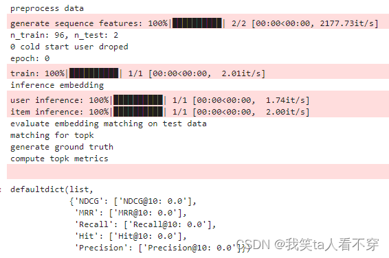

Task 2

The motivation of the DIN model: the traditional neural network model does not consider what the previous user’s historical behavior is, and which of the user’s historical behavior will have a positive effect on the current click prediction. In fact, whether the user clicks on the current product advertisement depends largely on his historical behavior. Mr. Wang Zhe gave an example

In order to better  express the user's broad and diverse interests,  we should consider the correlation between the user's historical behavior products and current product advertisements . If many of the user's historical products are associated with the current product, it means that the product may meet the user's taste. Just recommend the ad to him. When it comes to relevance, we can easily think of the idea of ​​"attention". Therefore, in order to better learn the relevance of the current product advertisement from the user's historical behavior and the change of the user's interest, the author uses Attention is introduced to the model, and a "local activation unit" structure is designed.

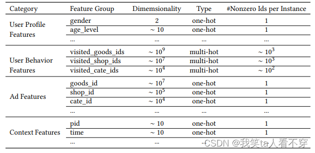
feature

Industrial CTR prediction data sets are generally in multi-group categorial formthe form of categorical features. This data set generally looks like this:

Base model 

The base model here is the form of Embedding&MLP mentioned above. The reason why this is introduced is because the benchmark of the DIN network is also him, but a new structure (attention network) is added on this basis to learn the current The correlation between the candidate advertisement and the user's historical behavior characteristics, so as to dynamically capture the user's interest.

The structure of the benchmark model is relatively simple. We have been using this benchmark before. It is divided into three modules: Embedding layer, Pooling & Concat layer and MLP. The structure is as follows:

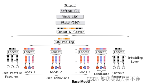
Embedding layer : The function of this layer is to convert the high-dimensional sparse input into a low-dimensional dense vector. Each discrete feature will correspond to an embedding dictionary. The dimension is D\times KD×K, where DD represents the hidden vector dimension, and KK represents the number of unique values ​​of the current discrete feature. For better understanding, here is an example, such as the above weekday feature:

Assuming that a user’s weekday feature is Friday, when it is converted into one-hot encoding, it is represented by [0,0,0,0,1,0,0]. Here, if the hidden vector dimension is assumed to be D, then this feature The corresponding embedding dictionary is a matrix of D\times7D×7 (each column represents an embedding, 7 columns exactly 7 embedding vectors, corresponding to Monday to Sunday), then the user's one-hot vector will be obtained after passing through the embedding layer A vector of D\times1D×1, which is the embedding corresponding to Friday, how to calculate it is actually the embedding matrix * [0,0,0,0,1,0,0]^Tembedding matrix∗[0,0 ,0,0,1,0,0]T . In fact, it is to directly take out the embedding vector at the position where the one-hot vector is 1 in the embedding matrix. In this way, a dense vector of sparse features is obtained. The same is true for other discrete features, except that the multi-hot code above will get a list of embedding vectors, because more than one of the multi-hot vectors he started is 1, so multiplying the embedding matrix will get A list is up. Through this layer, the above input features can get the corresponding dense embedding vector.

pooling layer and Concat layer : The role of the pooling layer is to convert the user's historical behavior embedding into a fixed-length vector, because the number of items purchased by each user is different, that is, in each user's multi-hot The number of 1 is inconsistent, so after the embedding layer, the number of user historical behavior embeddings obtained is not the same, that is, the above embedding list t_iti​is not the same length, then in this case, the historical behavior characteristics of each user are put together Not the same long. And if we add a fully connected network later, we know that he needs a fixed-length feature input. Therefore, a pooling layer is often used to first change the user's historical behavior embedding into a fixed length (uniform length), so there is this formula:

e_i=pooling(e_{i1}, e_{i2}, ...e_{ik})ei=pooling(ei1​,ei2​,...eik​)

Here e_{ij}eij​is the embedding of the user's historical behavior. e_iei​becomes a fixed-length vector, where ii represents the ii-th historical feature group (historical behavior, such as historical commodity id, historical commodity category id, etc.), and kk here represents the user in the corresponding historical special group The number of purchased products, that is, the number of historical embeddings, see the user behaviors series in the above picture, that is the process. The role of the Concat layer is to concatenate all the feature embedding vectors, if there are continuous features, they are also counted, spliced ​​and integrated from the feature dimension, and used as the input of MLP.

MLP : This is an ordinary full connection, which uses various interactions between learning features.

Loss : Since this is a click-through rate prediction task and a two-category problem, the loss function here uses a negative log logarithmic likelihood:

This is the whole picture of the base model. You should be able to see the problem of this model here. It can also be seen from the above figure that the user's historical behavior characteristics and current candidate advertisement characteristics are a little interaction before they are all put together for the neural network. There is no process, and after putting together to give the neural network, although there is interaction, some original information, for example, the information of each historical product will be lost, because the interaction with the current candidate advertising product is the pool The embedding of historical features after transformation, this embedding is a combination of all historical product information, this through our previous analysis, for predicting the current advertising click rate, not all historical products are useful, and the integration of all product information will add some noise Sexual information, you can think of the keyboard and mouse example mentioned above, if you add various facial cleansers, clothes and so on will have a counterproductive effect. Secondly, combined in this way, it is no longer possible to see which product in the user's historical behavior is more related to the current product, that is, the importance of each product in the historical behavior to the current prediction is lost. The last point is that if all the historical behavioral products browsed by users are finally converted into fixed-length embeddings through embedding and pooling, this will limit the model to learn the diverse interests of users.

So what are the ideas to improve this problem? The first is to increase the dimension of embedding and increase the expressive ability of each product before, so that even if it is combined, the expressive ability of embedding will be strengthened, and it can contain the user's interest information. However, the calculation amount in large-scale real recommendation scenarios is super Big, not desirable. Another idea is to introduce an attention mechanism between the current candidate advertisement and the user's historical behavior , so that when predicting whether the current advertisement is clicked, the model will pay more attention to those user history products related to the current advertisement, that is to say, the same as The more relevant historical behavior of the current product can promote the user's click behavior . Here is another example from the author:

Imagine a young mother visiting an e-commerce site, seeing a cute new handbag on display, and clicking on it. Let's analyze the drivers of click behavior.

The ad shown hits the young mother's relevant interests by soft-searching her historical behavior and discovering that she has recently viewed similar items such as tote bags and purses

The second idea is the improvement of DIN. DIN models this process by being given a candidate ad and then paying attention to representations of local interests related to that ad. Instead of expressing different interests of all users by using the same vector, DIN adaptively computes a representation vector of user interest (for a given ad) by considering the relevance of historical behavior. This representation vector varies from advertisement to advertisement. Let's take a look at the DIN model.

Torch-Rechub Tutorial： DeepFM

• Scenario: Fine row (CTR prediction)
• Model: DeepFM

• Data: Criteo Advertising Dataset

This dataset is an online advertising dataset released by Criteo Labs. It contains millions of click feedback records for display ads, which can be used as a benchmark for click-through rate (CTR) prediction. The dataset has 40 features, the first column is the label, where a value of 1 means the ad was clicked and a value of 0 means the ad was not clicked. Other features include 13 dense features and 26 sparse features.

import numpy as np
import pandas as pd
import torch
from torch_rechub.models.ranking import WideDeep, DeepFM, DCN
from torch_rechub.trainers import CTRTrainer
from torch_rechub.basic.features import DenseFeature, SparseFeature
from torch_rechub.utils.data import DataGenerator
from tqdm import tqdm
from sklearn.preprocessing import MinMaxScaler, LabelEncoder
torch.manual_seed(2022) #固定随机种子

data_path = 'criteo_sample.csv'
data = pd.read_csv(data_path)  
#data = pd.read_csv(data_path, compression="gzip") #if the raw_data is .gz file
data.head()

feature engineering

• Dense features: Also known as numerical features, such as salary and age. In this tutorial, two operations are performed on Dense features:
  • MinMaxScaler is normalized so that its value is between [0,1]
  • Discretize it into a new Sparse feature
• Sparse features: also known as category-type features, such as gender and education. In this tutorial, the LabelEncoder encoding operation is directly performed on the Sparse feature, and the original category string is mapped to a value, and the Embedding vector will be generated for each value in the model.

dense_cols= [f for f in data.columns.tolist() if f[0] == "I"] #以I开头的特征名为dense特征
sparse_cols = [f for f in data.columns.tolist() if f[0] == "C"]  #以C开头的特征名为sparse特征

data[dense_cols] = data[dense_cols].fillna(0) #填充空缺值
data[sparse_cols] = data[sparse_cols].fillna('-996')


#criteo比赛冠军分享的一种离散化思路，不用纠结其原理，大家也可以试试别的离散化手段
def convert_numeric_feature(val):
    v = int(val)
    if v > 2:
        return int(np.log(v)**2)
    else:
        return v - 2
        
for col in tqdm(dense_cols):  #将离散化dense特征列设置为新的sparse特征列
    sparse_cols.append(col + "_sparse")
    data[col + "_sparse"] = data[col].apply(lambda x: convert_numeric_feature(x))

scaler = MinMaxScaler()  #对dense特征列归一化
data[dense_cols] = scaler.fit_transform(data[dense_cols])

for col in tqdm(sparse_cols):  #sparse特征编码
    lbe = LabelEncoder()
    data[col] = lbe.fit_transform(data[col])

#重点：将每个特征定义为torch-rechub所支持的特征基类，dense特征只需指定特征名，sparse特征需指定特征名、特征取值个数(vocab_size)、embedding维度(embed_dim)
dense_features = [DenseFeature(feature_name) for feature_name in dense_cols]
sparse_features = [SparseFeature(feature_name, vocab_size=data[feature_name].nunique(), embed_dim=16) for feature_name in sparse_cols]
y = data["label"]
del data["label"]
x = data

training model

To train a DeepFM model, you only need to specify the DeepFM model structure parameters, learning rate and other training parameters. For DeepFM, the main parameters are as follows:

• deep_features refers to the features trained with the deep module (compatible with dense and sparse),
• fm_features refers to the features trained by the fm module, which can only be passed in the sparse type
• mlp_params specifies the parameters of the MLP layer in the deep module

# 构建模型输入所需要的dataloader，区分验证集、测试集，指定batch大小
#split_ratio=[0.7,0.1] 指的是训练集占比70%，验证集占比10%，剩下的全部为测试集
dg = DataGenerator(x, y) 
train_dataloader, val_dataloader, test_dataloader = dg.generate_dataloader(split_ratio=[0.7, 0.1], batch_size=256, num_workers=8)

from torch_rechub.models.ranking import DeepFM
from torch_rechub.trainers import CTRTrainer
#定义模型
model = DeepFM(
        deep_features=dense_features+sparse_features,
        fm_features=sparse_features,
        mlp_params={"dims": [256, 128], "dropout": 0.2, "activation": "relu"},
    )

# 模型训练，需要学习率、设备等一般的参数，此外我们还支持earlystoping策略，及时发现过拟合
ctr_trainer = CTRTrainer(
    model,
    optimizer_params={"lr": 1e-4, "weight_decay": 1e-5},
    n_epoch=1,
    earlystop_patience=3,
    device='cpu', #如果有gpu，可设置成cuda:0
    model_path='./', #模型存储路径
)
ctr_trainer.fit(train_dataloader, val_dataloader)

# 查看在测试集上的性能
auc = ctr_trainer.evaluate(ctr_trainer.model, test_dataloader)
print(f'test auc: {auc}')

Train Criteo with other ranking models

#定义相应的模型，用同样的方式训练
model = WideDeep(wide_features=dense_features, deep_features=sparse_features, mlp_params={"dims": [256, 128], "dropout": 0.2, "activation": "relu"})

model = DCN(features=dense_features + sparse_features, n_cross_layers=3, mlp_params={"dims": [256, 128]})

From tuning packages to customizing your own models

Congratulations to my friend for successfully running the DeepFM model and getting the result recommended by CTR. Next we consider how to implement our own DeepFM model. Since basic modules such as FM, MLP, LR, and Embedding are shared by many recommendation models, torch_rechub also helps us integrate these small modules. We can import it in basic.layers.

from torch_rechub.basic.layers import FM, MLP, LR, EmbeddingLayer

class MyDeepFM(torch.nn.Module):
  # Deep和FM为两部分，分别处理不同的特征，因此传入的参数要有两种特征，由此我们得到参数deep_features,fm_features
  # 此外神经网络类的模型中，基本组成原件为MLP多层感知机，多层感知机的参数也需要传进来，即为mlp_params
  def __init__(self, deep_features, fm_features, mlp_params):
    super().__init__()
    self.deep_features = deep_features
    self.fm_features = fm_features
    self.deep_dims = sum([fea.embed_dim for fea in deep_features])
    self.fm_dims = sum([fea.embed_dim for fea in fm_features])
    # LR建模一阶特征交互
    self.linear = LR(self.fm_dims)
    # FM建模二阶特征交互
    self.fm = FM(reduce_sum=True)
    # 对特征做嵌入表征
    self.embedding = EmbeddingLayer(deep_features + fm_features)
    self.mlp = MLP(self.deep_dims, **mlp_params)

  def forward(self, x):
    input_deep = self.embedding(x, self.deep_features, squeeze_dim=True)  #[batch_size, deep_dims]
    input_fm = self.embedding(x, self.fm_features, squeeze_dim=False)  #[batch_size, num_fields, embed_dim]

    y_linear = self.linear(input_fm.flatten(start_dim=1))
    y_fm = self.fm(input_fm)
    y_deep = self.mlp(input_deep)  #[batch_size, 1]
    # 最终的预测值为一阶特征交互，二阶特征交互，以及深层模型的组合
    y = y_linear + y_fm + y_deep
    # 利用sigmoid来将预测得分规整到0,1区间内
    return torch.sigmoid(y.squeeze(1))

Similarly, you can use the trainer provided by torch-rechub for model training and model evaluation

model = MyDeepFM(
        deep_features=dense_features+sparse_features,
        fm_features=sparse_features,
        mlp_params={"dims": [256, 128], "dropout": 0.2, "activation": "relu"},
    )
# 模型训练，需要学习率、设备等一般的参数，此外我们还支持earlystoping策略，及时发现过拟合
ctr_trainer = CTRTrainer(
    model,
    optimizer_params={"lr": 1e-4, "weight_decay": 1e-5},
    n_epoch=1,
    earlystop_patience=3,
    device='cpu',
    model_path='./',
)
ctr_trainer.fit(train_dataloader, val_dataloader)

# 查看在测试集上的性能
auc = ctr_trainer.evaluate(ctr_trainer.model, test_dataloader)
print(f'test auc: {auc}')

Torch-Rechub Tutorial: DIN

Task 1

First of all, the dataset we use is: amazon_electronics_sample.csv

It mainly contains 4 features: user_id (user id), item_id (click product id), cate_id (click product category id), time (time series)

Read data and feature engineering, Sparse category Dense numeric 

Sequence features : Sequence features, such as user historical click item_id sequence, historical store sequence, etc. How to extract sequence features is a key point of our study in DIN, and it is also one of the main innovation points of DIN.

import torch
import torch_rechub
import pandas as pd
import tqdm
import sklearn
torch.manual_seed(2022)

file_path = 'amazon_electronics_sample.csv'#'amazon_electronic_datasets.csv'
data = pd.read_csv(file_path)
data.head()

# 构建用户的历史行为序列特征，内置函数create_seq_features只需要指定数据，
# 和需要生成序列的特征，drop_short是选择舍弃行为序列较短的用户
from torch_rechub.utils.data import create_seq_features
train, val, test = create_seq_features(data, seq_feature_col=['item_id', 'cate_id'], drop_short=0)

from torch_rechub.basic.features import DenseFeature, SequenceFeature, SparseFeature
n_users, n_items, n_cates = data['user_id'].max(), data['item_id'].max(), data['cate_id'].max()
features = [SparseFeature("target_item", vocab_size=n_items + 2, embed_dim=8),
            SparseFeature('target_cate', vocab_size=n_cates + 2, embed_dim=8),
            SparseFeature('user_id', vocab_size=n_users + 2, embed_dim=8)]
target_features = features

# 对于序列特征，除了需要和类别特征一样处理意外，item序列和候选item应该属于同一个空间，我们希望模
# 型共享它们的embedding，所以可以通过shared_with参数指定

history_features = [
    SequenceFeature('history_item', vocab_size=n_items+2, embed_dim=8, pooling='concat', shared_with='target_item'),
    SequenceFeature('history_cate', vocab_size=n_items+2, embed_dim=8, pooling='concat', shared_with='target_cate'),
]

out:

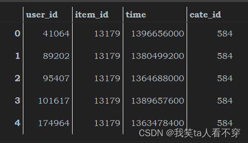
[<torch_rechub.basic.features.SparseFeature at 0x2349895ecc8>,
 <torch_rechub.basic.features.SparseFeature at 0x2349895e508>,
 <torch_rechub.basic.features.SparseFeature at 0x2349895ee08>]

The vocab_size=n_items+2 here needs to be added +2 for OOV (out-of-vocabulary) tags and padding (filling) after online query.

Here embed_dim=8 is an empirical parameter.

from torch_rechub.utils.data import df_to_dict, DataGenerator
# 指定 label 生成模型输入
train = df_to_dict(train)
val = df_to_dict(val)
test = df_to_dict(test)

train_y, val_y, test_y = train['label'], val['label'], test['label']

del train["label"]
del val["label"]
del test["label"]

train_x, val_x, test_x = train, val, test
# 最后查看一次输入模型的数据格式
train_x

out:

{'user_id': array([1, 1]),
 'history_item': array([[2, 3, 0, 0, 0, 0, 0, 0, 0, 0, 0, 0, 0, 0, 0, 0, 0, 0, 0, 0, 0, 0,
         0, 0, 0, 0, 0, 0, 0, 0, 0, 0, 0, 0, 0, 0, 0, 0, 0, 0, 0, 0, 0, 0,
         0, 0, 0, 0, 0, 0],
        [2, 3, 0, 0, 0, 0, 0, 0, 0, 0, 0, 0, 0, 0, 0, 0, 0, 0, 0, 0, 0, 0,
         0, 0, 0, 0, 0, 0, 0, 0, 0, 0, 0, 0, 0, 0, 0, 0, 0, 0, 0, 0, 0, 0,
         0, 0, 0, 0, 0, 0]]),
 'history_cate': array([[2, 4, 0, 0, 0, 0, 0, 0, 0, 0, 0, 0, 0, 0, 0, 0, 0, 0, 0, 0, 0, 0,
         0, 0, 0, 0, 0, 0, 0, 0, 0, 0, 0, 0, 0, 0, 0, 0, 0, 0, 0, 0, 0, 0,
         0, 0, 0, 0, 0, 0],

# 构建dataloader  指定模型读取数据的方式， 和区分验证集测试集，指定batch_size
dg = DataGenerator(train_x, train_y)
train_dataloader, val_dataloader, test_dataloader = dg.generate_dataloader(x_val=val_x, y_val=val_y, x_test=test_x, y_test=test_y, batch_size=16)

from torch_rechub.models.ranking import DIN
from torch_rechub.trainers import CTRTrainer

# 定义模型，模型的参数需要我们之前的feature类，用于构建模型的输入层，mlp指定模型后续DNN的结构，attention_mlp指定attention层的结构
model = DIN(features=features, history_features=history_features, target_features=target_features, mlp_params={"dims": [256, 128]}, attention_mlp_params={"dims": [256, 128]})

# 模型训练，需要学习率、设备等一般的参数，此外我们还支持earlystoping策略，及时发现过拟合
ctr_trainer = CTRTrainer(model, optimizer_params={"lr": 1e-3, "weight_decay": 1e-3}, n_epoch=3, earlystop_patience=4, device='cpu', model_path='./')
ctr_trainer.fit(train_dataloader, val_dataloader)

# 查看在测试集上的性能
auc = ctr_trainer.evaluate(ctr_trainer.model, test_dataloader)
print(f'test auc: {auc}')

out:

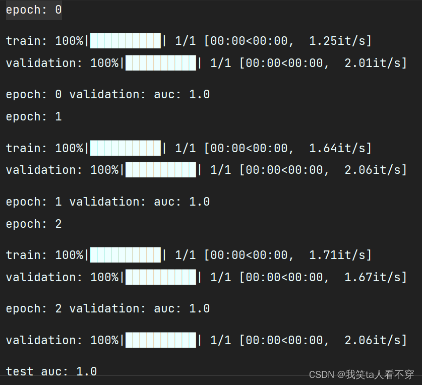
 This content is learned from:

torch-rechub/DIN.ipynb at main · datawhalechina/torch-rechub · GitHubhttps://github.com/datawhalechina/torch-rechub/blob/main/tutorials/DIN.ipynb