Harbin Institute of Technology 2022 Machine Learning Experiment 1: Curve Fitting

The requirements of this experiment are quite clear (compared to the previous semester). This blog is implemented in python, the scientific computing library is used numpy, and the drawing is used matplotlib.pyplot. For simplicity, import the following at the beginning of the file:

import numpy as np
import matplotlib.pyplot as plt

The numpy functions used in this experiment

Generally numpyabbreviated as np(import numpy as np). The following is a brief introduction to the numpy functions used in the experiment. The following code needs to be added at the top import numpy as np.

np.array

This function returns an numpy.ndarrayobject, which can be understood as a multi-dimensional array (only one-dimensional (can be regarded as a column vector) and two-dimensional (matrix) will be used in this experiment). Use lowercase $xx$ is a column vector, uppercase$A$ represents a matrix. A.TmeansAATranspose of$A.$The operations on pairsndarrayare generally element-wise.

>>> x = np.array([1,2,3])
>>> x
array([1, 2, 3])
>>> A = np.array([[2,3,4],[5,6,7]])
>>> A
array([[2, 3, 4],
       [5, 6, 7]])
>>> A.T # 转置
array([[2, 5],
       [3, 6],
       [4, 7]])
>>> A + 1
array([[3, 4, 5],
       [6, 7, 8]])
>>> A * 2
array([[ 4,  6,  8],
       [10, 12, 14]])

np.random

np.randomThe module contains several functions for generating random numbers. In this experiment, random initialization parameters (gradient descent method) are used to add noise to the data.

>>> np.random.rand(3, 3) # 生成3 * 3 随机矩阵，每个元素服从[0,1)均匀分布
array([[8.18713933e-01, 5.46592778e-01, 1.36380542e-01],
       [9.85514865e-01, 7.07323389e-01, 2.51858374e-04],
       [3.14683662e-01, 4.74980699e-02, 4.39658301e-01]])
      
>>> np.random.rand(1) # 生成单个随机数
array([0.70944563])
>>> np.random.rand(5) # 长为5的一维随机数组
array([0.03911319, 0.67572368, 0.98884287, 0.12501456, 0.39870096])
>>> np.random.randn(3, 3) # 同上，但每个元素服从N(0, 1)（标准正态）

math function

Only used in this experiment np.sin. These mathematical functions np.ndarrayoperate element-wise:

>>> x = np.array([0, 3.1415, 3.1415 / 2]) # 0, pi, pi / 2
>>> np.round(np.sin(x)) # 先求sin再四舍五入: 0, 0, 1
array([0., 0., 1.])

In addition, there are np.logfunctions similar np.expto python's mathlibrary (only for element-wise operations on multidimensional arrays).

np.dot

Returns the product of two matrices. Consistent with matrix multiplication in linear algebra. The columns of the first matrix are required to be equal to the number of rows of the second matrix. In particular, when one of them is a one-dimensional array, the shape is automatically adapted to $n\times 1$ or$1\times n.$

>>> x = np.array([1,2,3]) # 一维数组
>>> A = np.array([[1,1,1],[2,2,2],[3,3,3]]) # 3 * 3矩阵
>>> np.dot(x,A)
array([14, 14, 14])
>>> np.dot(A,x)
array([ 6, 12, 18])

>>> x_2D = np.array([[1,2,3]]) # 这是一个二维数组（1 * 3矩阵）
>>> np.dot(x_2D, A) # 可以运算
array([[14, 14, 14]])
>>> np.dot(A, x_2D) # 行列不匹配
Traceback (most recent call last):
  File "<stdin>", line 1, in <module>
  File "<__array_function__ internals>", line 5, in dot
ValueError: shapes (3,3) and (1,3) not aligned: 3 (dim 1) != 1 (dim 0)

np.eye

np.eye(n)Returns a unit matrix of order n.

>>> A = np.eye(3)
>>> A
array([[1., 0., 0.],
       [0., 1., 0.],
       [0., 0., 1.]])

Linear Algebra Correlation

np.linalgis a library related to linear algebra.

>>> A
array([[1, 0, 0],
       [0, 2, 0],
       [0, 0, 3]])
>>> np.linalg.inv(A) # 求逆（本实验不考虑逆不存在）
array([[1.        , 0.        , 0.        ],
       [0.        , 0.5       , 0.        ],
       [0.        , 0.        , 0.33333333]])
>>> x = np.array([1,2,3])
>>> np.linalg.norm(x) # 返回向量x的模长（平方求和开根号）
3.7416573867739413
>>> np.linalg.eigvals(A) # A的特征值
array([1., 2., 3.])

Generate data

Generating the data requires adding noise (error). The example given in class is the sine function, we also use the standard sine function $Y=\sin x.$ (After adding noise, it is$Y=\sin x+ϵ,$ with$ϵ\sim N(0,p^2)$, since$\sin$The maximum value of$x$$1$ , we set the variance of the error to be smaller, here it is set to$\frac{}{25}$).

'''
返回数据集，形如[[x_1, y_1], [x_2, y_2], ..., [x_N, y_N]]
保证 bound[0] <= x_i < bound[1].
- N 数据集大小, 默认为 100
- bound 产生数据横坐标的上下界, 应满足 bound[0] < bound[1], 默认为(0, 10)
'''
def get_dataset(N = 100, bound = (0, 10)):
    l, r = bound
    # np.random.rand 产生[0, 1)的均匀分布，再根据l, r缩放平移
    # 这里sort是为了画图时不会乱，可以去掉sorted试一试
    x = sorted(np.random.rand(N) * (r - l) + l)
	
	# np.random.randn 产生N(0,1)，除以5会变为N(0, 1 / 25)
    y = np.sin(x) + np.random.randn(N) / 5
    return np.array([x,y]).T

The resulting dataset has a point on a plane per row. The resulting data looks like this:

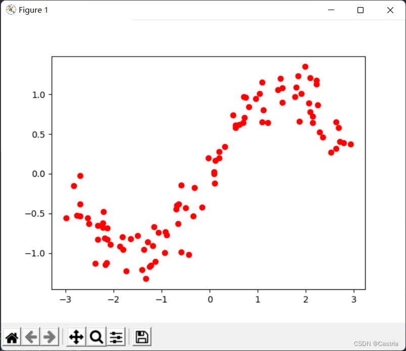
vaguely in the shape of a sine function. The code that produces the above image is as follows:

dataset = get_dataset(bound = (-3, 3))
# 绘制数据集散点图
for [x, y] in dataset:
    plt.scatter(x, y, color = 'red')
plt.show()

Least Squares Fitting

Below we use four methods (least squares, regular term/ridge regression, gradient descent, conjugate gradient) to fit the above perturbed sinusoids with polynomials.

Analytical solution derivation

Simply recall the principle of the least squares method: now we want to use a mmPolynomial$f\; (\; x\; )\; of\; degree\; m$
$$f(x)={in}_{}+{in}_{}x+{in}_{}{x}^2+...+{in}_m{x}^m$$
to approximate the true function$Y=\sin x.$ Our goal is to minimize the datasets$(x_{},Y_{}),(x_{},Y_{}),...,(x_N,Y_N)$ on the loss$L$ (loss), where the loss function takes the squared error:
$$L=\sum _{i=1}^N[{and}_i-f(x_i){]}^2$$
In order to find the parameters${in}_{},{in}_{},...,{in}_m,$ we need to find the loss$L$ related to w 0 , w 1 , . . . , wm w_0, w_1,...,w_m${in}_{},{in}_{},...,{in}_m$derivative of . For convenience, we use linear algebra notation:
$$X={⎝\begin{array}{ccccc}1& x_{}& x_1^{}& \cdots & x_1^m\\ 1& x_{}& x_2^{}& \cdots & x_2^m\\ ⋮& & & & ⋮\\ & x_N& x_N^{}& & x_N^m\end{array}⎠}_{N\times (m+1)},Y={⎝\begin{array}{c}{Y}_{}\\ Y_{}\\ ⋮\\ Y_N\end{array}⎠}_{N\times },In={⎝\begin{array}{c}{in}_{}\\ {in}_{}\\ ⋮\\ {in}_m\end{array}⎠}_{(m+1)\times 1}.$$
Under this representation,
$$⎝\begin{array}{c}f(x_{})\\ f\left(x_{}\right)\\ ⋮\\ f(x_N\end{array}⎠=XW.$$
If you have any doubts, you can verify it yourself with matrix multiplication. Continuing, the sum of the error terms can be expressed as
$$⎝\begin{array}{c}f\left(x_{}\right)-Y_{}\\ f\left(x_{}\right)-Y_{}\\ ⋮\\ f\left(x_N\right)-Y_N\end{array}⎠=XW-Y.$$
Therefore, the loss function
$$L=(XW-and{)}^T(XW-Y).$$
(To find the vector$xx=(x_{},x_{},...,x_N{)}^{}$The sum of the squares of the components of${}^T$$xx$ is the inner product, that is,${xx}^{T}xx.$ )
in order to obtain the$L$ smallest$W$ (this$W$ is a column vector), we needtoFind the partial derivative of$L$$0:$
$$\begin{array}{rl}\frac{\partial }{\partial W}& =\frac{}{\partial W}[(XW-and{)}^T(XW-Y)]\\ & =\frac{}{\partial W}[(W^T{X}^T-Y^T)(XW-Y)]\\ & =\frac{}{\partial W}({W.}^T{X}^{T}XW-{In}^T{X}^{T}Y-Y^{T}XW+Y^{T}Y)\\ & =\frac{}{\partial W}({W.}^T{X}^{T}XW-2Y^{T}XW+Y^{T}Y)(easy\; to\; verify,{In}^T{X}^{T}Y=Y^{T}XW,thus\; can\; be\; combined)\\ & =2X^{T}XW-2X^T\end{array}$$
Description:
(1) From line 3 to line 4, due to ${In}^T{X}^{T}Y$和$Y^{T}XW$are all numbers (or$1\times 1$ matrix), the two are transposed of each other, so the values ​​are the same and can be combined into one item.
(2) Derivation of the matrix from row 4 to row 5, the first term$\frac{}{\partial W}({W.}^T(X^{T}X\left)W\right)$is about$The\; quadratic\; form\; of\; W$ , its derivative is$2X^{T}XW.$
(3) For the primary term$-2Y^{The\; derivation\; of\; T}XW$, if the derivation according to the real number field, should get$-2Y^{T}X.$But check and find that the type of the matrix is ​​not correct, you need to do a transposition, it becomes$-2X^{T}Y.$

Matrix linear algebra has not been taught systematically in the class, only to explain what appears here. ( I won't if there are more )
Let the partial derivative be 0, get
$$X^{T}XW=Y^{T}X,$$
left multiply$(X^{T}X{)}^{-1}$（$X^{}$See the supplementary note below for the reversibility of${}^T$$X$
$$In=(X^{T}X{)}^{-1}{X}^{T}Y.$$
This is the$For\; the\; analytical\; solution\; of\; W$ , we only need to call the function to calculate this value.

'''
最小二乘求出解析解, m 为多项式次数
最小二乘误差为 (XW - Y)^T*(XW - Y)
- dataset 数据集
- m 多项式次数, 默认为 5
'''
def fit(dataset, m = 5):
    X = np.array([dataset[:, 0] ** i for i in range(m + 1)]).T
    Y = dataset[:, 1]
    return np.dot(np.dot(np.linalg.inv(np.dot(X.T, X)), X.T), Y)

Explain the code a little: the first line generates the $The\; X$ matrix,dataset[:,0]which is the 0th column of the dataset$(x_{},x_{},...,x_N{)}^T$ ; the second line is$Y$ matrix; the third row returns the analytical solution above. (If you are not familiar with python syntax ornumpylibraries, it is quite unfriendly)

Simply verify the result of the function we have completed: To do this, we first write a drawfunction to convert the obtained WWThe polynomialf ( x ) f(x)$corresponding\; to\; W$Draw$f$$($$x$$)$pyplot onto the library image:

'''
绘制给定系数W的, 在数据集上的多项式函数图像
- dataset 数据集
- w 通过上面四种方法求得的系数
- color 绘制颜色, 默认为 red
- label 图像的标签
'''
def draw(dataset, w, color = 'red', label = ''):
    X = np.array([dataset[:, 0] ** i for i in range(len(w))]).T
    Y = np.dot(X, w)
    
    plt.plot(dataset[:, 0], Y, c = color, label = label)

Then the main function:

if __name__ == '__main__':
    dataset = get_dataset(bound = (-3, 3))
    # 绘制数据集散点图
    for [x, y] in dataset:
        plt.scatter(x, y, color = 'red')
    # 最小二乘
    coef1 = fit(dataset)
    draw(dataset, coef1, color = 'black', label = 'OLS')
    
	# 绘制图像
    plt.legend()
    plt.show()

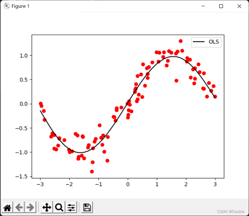
It can be seen that the effect of the 5th degree polynomial fitting is quite good (the data set is randomly generated each time, so it is different from the first picture).

As of all the code in this part, the following functions of the same name are no longer described:

import numpy as np
import matplotlib.pyplot as plt

'''
返回数据集，形如[[x_1, y_1], [x_2, y_2], ..., [x_N, y_N]]
保证 bound[0] <= x_i < bound[1].
- N 数据集大小, 默认为 100
- bound 产生数据横坐标的上下界, 应满足 bound[0] < bound[1]
'''
def get_dataset(N = 100, bound = (0, 10)):
    l, r = bound
    x = sorted(np.random.rand(N) * (r - l) + l)
    y = np.sin(x) + np.random.randn(N) / 5
    return np.array([x,y]).T

'''
最小二乘求出解析解, m 为多项式次数
最小二乘误差为 (XW - Y)^T*(XW - Y)
- dataset 数据集
- m 多项式次数, 默认为 5
'''
def fit(dataset, m = 5):
    X = np.array([dataset[:, 0] ** i for i in range(m + 1)]).T
    Y = dataset[:, 1]
    return np.dot(np.dot(np.linalg.inv(np.dot(X.T, X)), X.T), Y)
'''
绘制给定系数W的, 在数据集上的多项式函数图像
- dataset 数据集
- w 通过上面四种方法求得的系数
- color 绘制颜色, 默认为 red
- label 图像的标签
'''
def draw(dataset, w, color = 'red', label = ''):
    X = np.array([dataset[:, 0] ** i for i in range(len(w))]).T
    Y = np.dot(X, w)
    
    plt.plot(dataset[:, 0], Y, c = color, label = label)

if __name__ == '__main__':

    dataset = get_dataset(bound = (-3, 3))
    # 绘制数据集散点图
    for [x, y] in dataset:
        plt.scatter(x, y, color = 'red')
    
    coef1 = fit(dataset)
    draw(dataset, coef1, color = 'black', label = 'OLS')

    plt.legend()
    plt.show()

Supplementary Instructions

There is a less rigorous piece above: for a matrix $For\; X$ ,$X^{T}X$is not necessarily reversible. In this experiment, however, it can be shown that it is an invertible matrix. Since this class is not a linear algebra class, we won't spend too much space on this, just a brief reminder:
(1)$X$ is an$N\times (m+1)$ of the matrix. where the number of data is$N$ is much larger than the polynomial degree$m$ , there are$N>m+1;$
(2) To illustrate$X^{T}X$is invertible, need to explain$(X^{T}X{)}_{(m+1)\times (m+1)}$Full rank, that is, $R(X^{T}X)=m+1;$
(3) In linear algebra, we have proved that$R(X)=R(X^T)=R\left(X^{T}X\right)=R(X{X}^T);$
（4）$X$ is aVandermonde matrixwhose rank is equal to$my\{N,m+1\}=m+1.$

Add regularization term (ridge regression)

The least squares method is prone to overfitting. In order to illustrate this defect, we use the first 50 points of the generated data set for training (so that the sampling is not uniform enough, here is just to illustrate the overfitting), obtain the parameters, and then draw the entire function image to check the fitting effect:

if __name__ == '__main__':
    dataset = get_dataset(bound = (-3, 3))
    # 绘制数据集散点图
    for [x, y] in dataset:
        plt.scatter(x, y, color = 'red')
    # 取前50个点进行训练
    coef1 = fit(dataset[:50], m = 3)
    # 再画出整个数据集上的图像
    draw(dataset, coef1, color = 'black', label = 'OLS')

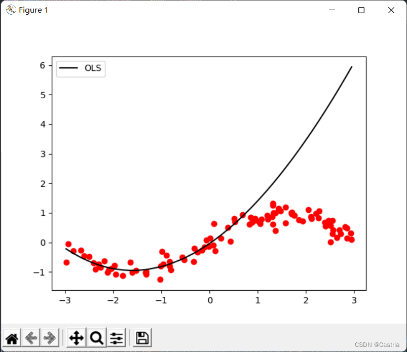
Overfitting in mmThis is especially serious when$m$$m=3$ o'clock). As the polynomial degree increases, in order to be as close as possible to the given data set, the magnitude of the calculated coefficients will be larger and larger, and the performance on unseen samples will be worse. As shown above, you can see that the fit is at the first 50 points (approximately on the abscissa$[-3,0]$ ) is very good; on the test set the performance is very poor ($[0,3]$ ). To prevent overfitting, a regularization term can be introduced. At this time, the loss function$L$变为
$$L=(XW-and{)}^T(XW-and)+\lambda ||W|{|}_2^{}$$
where $||\cdot |{|}_2^{}$Indicates $L_{}$The square of the norm, in this case ${In}^{T}W;\lambda$ is the regularization coefficient. This formula is also called Ridge Regression. Its idea is to take into account the loss function and the resulting parameter$Modulo\; length\; of\; W$ (at$L_{}$norm), preventing $The\; parameter\; in\; W$ is too large.

For example (numbers are made up randomly): when the regularization coefficient is $1$ , if the squared error of scheme 1 on the data set is$0.5,$ at this time$In=(100,-200,300,150{)}^T$ ; the squared error of scheme 2 on the dataset is$10,$ at this time$In=(1,-3,2,1)$ , then we choose$W.$ Regularization coefficient$\lambda$ characterizes this for$The\; importance\; of\; the\; W$ modulus length:λ \lambdaThe larger the$\lambda$$The\; higher\; the\; module\; length\; of\; W$ , the greater the penalty. When$l=0,\; the$ ridge regression becomes the ordinary least squares method. Similar to ridge regression is LASSO, which is to replace the regularization term with$L_{}$norm.

Repeating the above derivation, we can get the analytical solution as
$$In=(X^{T}X+\lambda E_{m+1}{)}^{-1}{X}^{T}Y.$$
where${AND}_{m+1}$is $m+1st$ order unit matrix. It is easy to get$(X^{T}X+\lambda E_{m+1})$ is also reversible.

This part of the code is as follows.

'''
岭回归求解析解, m 为多项式次数, l 为 lambda 即正则项系数
岭回归误差为 (XW - Y)^T*(XW - Y) + λ(W^T)*W
- dataset 数据集
- m 多项式次数, 默认为 5
- l 正则化参数 lambda, 默认为 0.5
'''
def ridge_regression(dataset, m = 5, l = 0.5):
    X = np.array([dataset[:, 0] ** i for i in range(m + 1)]).T
    Y = dataset[:, 1]
    return np.dot(np.dot(np.linalg.inv(np.dot(X.T, X) + l * np.eye(m + 1)), X.T), Y)

The comparison of the two methods is as follows:

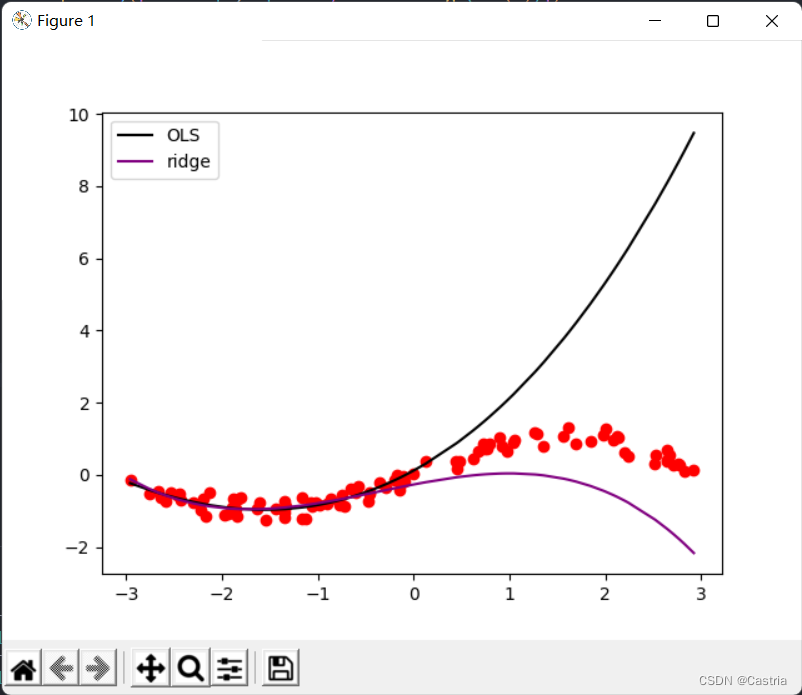
It can be seen from the comparison that ridge regression significantly reduces overfitting (at this time $m=3,l=0.3$ ).

Gradient Descent

Gradient descent is not the best way to solve this problem, and it can easily fail to converge. First briefly introduce the basic idea of ​​gradient descent method: if we want to find the complex function f ( x ) f(x)The minimum value (maximum point) of$f$$($$x$$)$$x$ may be a vector, etc.), i.e.
$$x_{min}=\underset{x}{\mathrm{argmin}}f\left(x\right)$$
gradient descent repeats the following operations:
(0) (randomly) initialize$x_{}(t=0)$ ;
(1) Let$f\left(x\right)$ in$x_t$gradient at (when $When\; x$ is one-dimensional, it is the derivative)$\nabla f(x_t)$；
（2）$x_{t+1}=x_t-\eta \nabla f(x_t)$
(3) If$x_{t+1}$with $x_t$If there is little difference (reaches the preset range) or the number of iterations reaches the preset upper limit, stop the algorithm; otherwise repeat (1) (2).

Among them η \ eta$\eta$ is the learning rate, which determines the step size of gradient descent.
The following is a gradient descent method to find$Y=x^{}$Example program for the minimum point of${}^{2\; :}$

import numpy as np
import matplotlib.pyplot as plt

def f(x):
    return x ** 2

def draw():
    x = np.linspace(-3, 3)
    y = f(x)
    plt.plot(x, y, c = 'red')

cnt = 0
# 初始化 x
x = np.random.rand(1) * 3
learning_rate = 0.05

while True:
    grad = 2 * x
    # -----------作图用，非算法部分-----------
    plt.scatter(x, f(x), c = 'black')
    plt.text(x + 0.3, f(x) + 0.3, str(cnt))
    # -------------------------------------
    new_x = x - grad * learning_rate
    # 判断收敛
    if abs(new_x - x) < 1e-3:
        break

    x = new_x
    cnt += 1

draw()
plt.show()

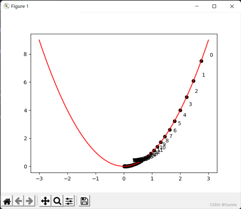
The picture above indicates $x$ As the iteration evolves, you can see$x$ keeps approaching zero along the positive semi-axis. It should be noted that the learning rate cannot be too large (although in the above program, the learning rate is set a little small), it needs to be adjusted manually, otherwise it is easy to imagine,$x$ oscillates back and forth on the positive and negative semi-axes, making it difficult to converge.

In least squares, the function we need to optimize is the loss function
$$L=(XW-and{)}^T(XW-Y).$$
Next we solve the problem with gradient descent. In the derivation above,
$$\begin{array}{r}\frac{\partial }{\partial W}=2X^{T}XW-2X^T\end{array},$$
so each time we perform an iteration on$W$ subtracts this gradient until parameter$W$ converges. However, after experiments, the squared error will make the gradient too large and the process cannot converge. Therefore, the mean squared error (MSE) is used to replace it, which is to divide the original formula by$N$:

'''
梯度下降法(Gradient Descent, GD)求优化解, m 为多项式次数, max_iteration 为最大迭代次数, lr 为学习率
注: 此时拟合次数不宜太高(m <= 3), 且数据集的数据范围不能太大(这里设置为(-3, 3)), 否则很难收敛
- dataset 数据集
- m 多项式次数, 默认为 3(太高会溢出, 无法收敛)
- max_iteration 最大迭代次数, 默认为 1000
- lr 梯度下降的学习率, 默认为 0.01
'''
def GD(dataset, m = 3, max_iteration = 1000, lr = 0.01):
    # 初始化参数
    w = np.random.rand(m + 1)

    N = len(dataset)
    X = np.array([dataset[:, 0] ** i for i in range(len(w))]).T
    Y = dataset[:, 1]

    try:
        for i in range(max_iteration):
            pred_Y = np.dot(X, w)
            # 均方误差（省略系数2）
            grad = np.dot(X.T, pred_Y - Y) / N
            w -= lr * grad
    '''
    为了能捕获这个溢出的 Warning，需要import warnings并在主程序中加上：
    warnings.simplefilter('error')
    '''
    except RuntimeWarning:
        print('梯度下降法溢出, 无法收敛')

    return w

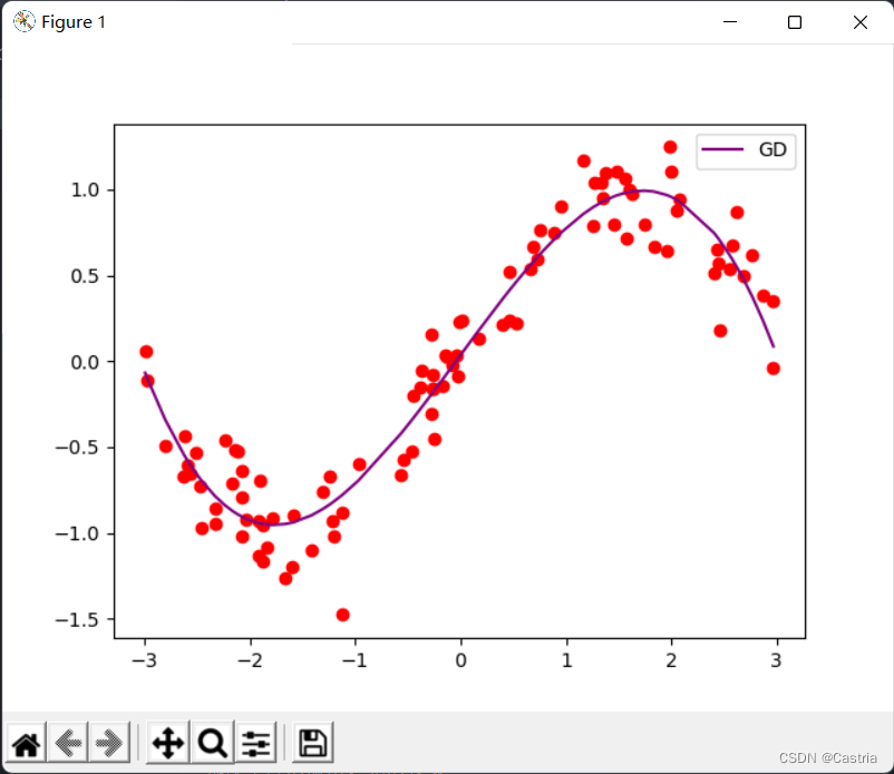
At this time if $If\; m$ is set a little larger (say 4), the gradient will overflow during the iteration, making the parameters unable to converge. When converging, the fitting effect is OK:

Conjugate gradient method

Conjugate Gradients can be used to solve the form $Axx=b$System of equations for$b$$f(xx)=\frac{}{2}{xx}^{T}Axx-{bb}^{T}xx+c.$ (It can be shown that for positive definite$A$ , the two are equivalent) where$A$ is apositive definitematrix. In this problem, we ask to solve$$X^{T}XW=Y^{T}X,$$
then$A_{(m+1)\times (m+1)}=X^{T}X,bb=Y^T.$If we want to add a regular term, it becomes the solution
$$(X^{T}X+\lambda E)W=Y^{T}X.$$
First of all, let me explain:$X^{T}X$is not necessarily positive definite but must be positive semi-definite (see). But in the experiment we basically don't have to worry about this problem, because$X^{T}X$is very likely to be positive definite, we only add an assertion to the code, and don't pay much attention to this condition.
The idea of ​​the conjugate gradient method and the proof process are relatively long. You can refer tothis series. Only the algorithm steps are given here (at the beginning of the third article linked above):

(0) Initialize $x_{(0};$
(1) Initialize$d_{(0}=r_{(0}=b-A{x}_{(0};$
（2）令$$a_{(i)}=\frac{r_{\left(i\right)}^T{r}_{\left(i\right)}}{d_{(i)}^{T}A{d}_{\left(i\right)}};$$
（3）迭代$x_{(i+1)}=x_{\left(i\right)}+a_{\left(i\right)}{d}_{\left(i\right)};$
（4）令$r_{(i+1)}=r_{\left(i\right)}-a_{\left(i\right)}A{d}_{\left(i\right)};$
（5）令$$b_{(i+1)}=\frac{r_{(i+1)}^T{r}_{(i+1)}}{r_{\left(i\right)}^T{r}_{\left(i\right)}},d_{(i+1)}=r_{(i+1)}+b_{(i+1)}{d}_{(i)}.$$
（6）当$\frac{||r_{\left(i\right)}}{||r_{(0}||}<ϵ$ , stop the algorithm; otherwise continue to iterate from (2). $ϵ$ is a small pre-set value, I take here$10^{-5.}Below\; we\; follow\; this\; process\; to$
implement the code:

'''
共轭梯度法(Conjugate Gradients, CG)求优化解, m 为多项式次数
- dataset 数据集
- m 多项式次数, 默认为 5
- regularize 正则化参数, 若为 0 则不进行正则化
'''
def CG(dataset, m = 5, regularize = 0):
    X = np.array([dataset[:, 0] ** i for i in range(m + 1)]).T
    A = np.dot(X.T, X) + regularize * np.eye(m + 1)
    assert np.all(np.linalg.eigvals(A) > 0), '矩阵不满足正定!'
    b = np.dot(X.T, dataset[:, 1])
    w = np.random.rand(m + 1)
    epsilon = 1e-5

    # 初始化参数
    d = r = b - np.dot(A, w)
    r0 = r
    while True:
        alpha = np.dot(r.T, r) / np.dot(np.dot(d, A), d)
        w += alpha * d
        new_r = r - alpha * np.dot(A, d)
        beta = np.dot(new_r.T, new_r) / np.dot(r.T, r)
        d = beta * d + new_r
        r = new_r
        # 基本收敛，停止迭代
        if np.linalg.norm(r) / np.linalg.norm(r0) < epsilon:
            break
    return w

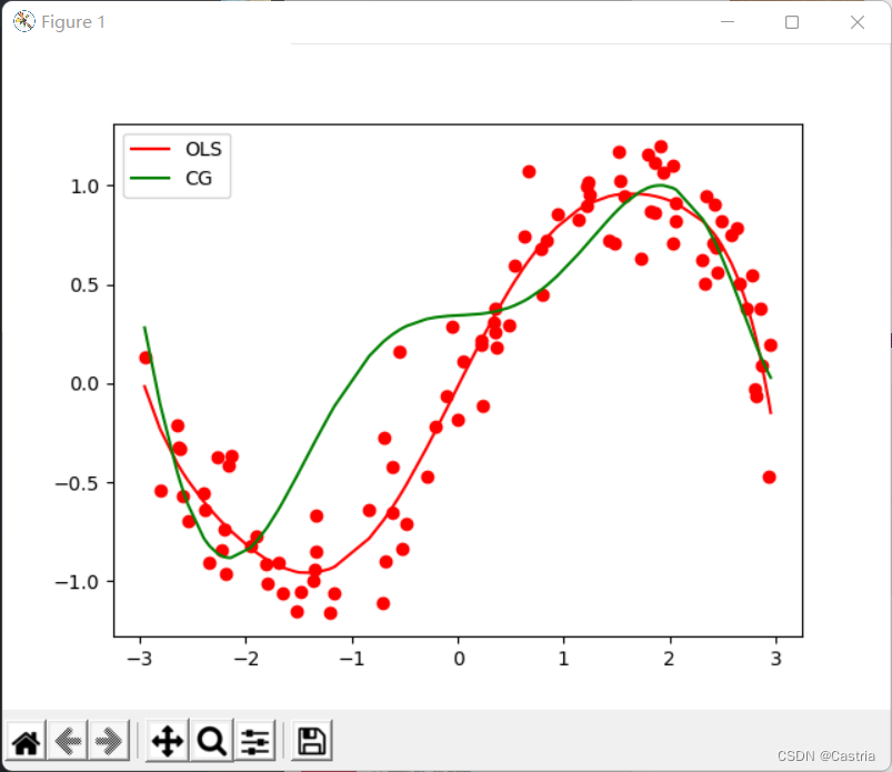
Compared with the naive gradient descent method, the conjugate gradient method converges quickly and stably. However, as the degree of the polynomial increases, the fit becomes worse: at $m=7$ , it is compared with the least squares method as follows:

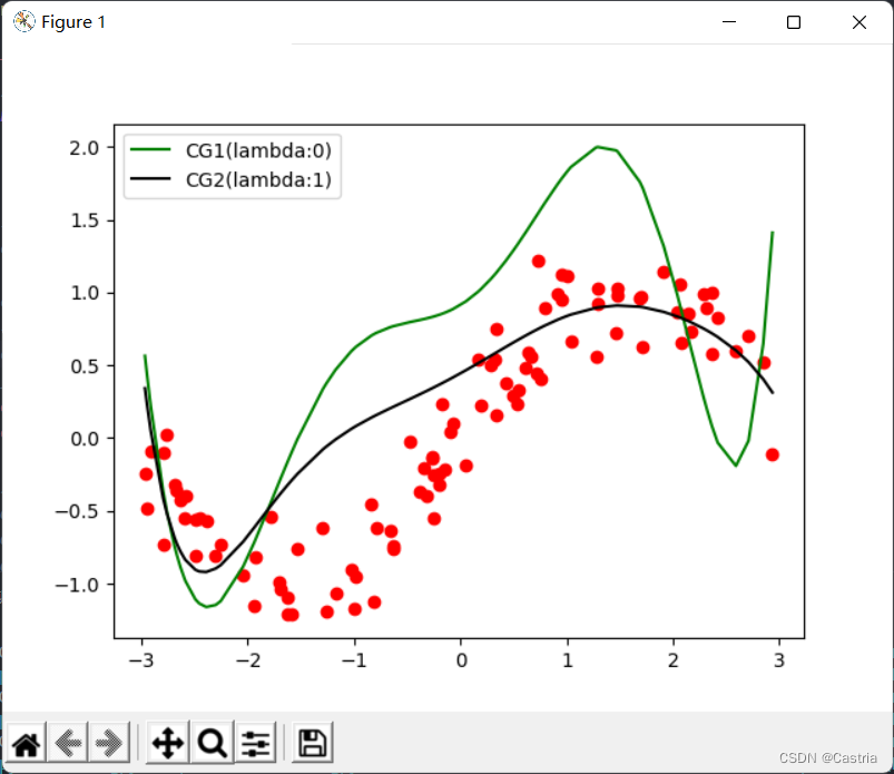
At this time, it can still be partially alleviated by the regular term (the figure is$m=7,l=1$ ):

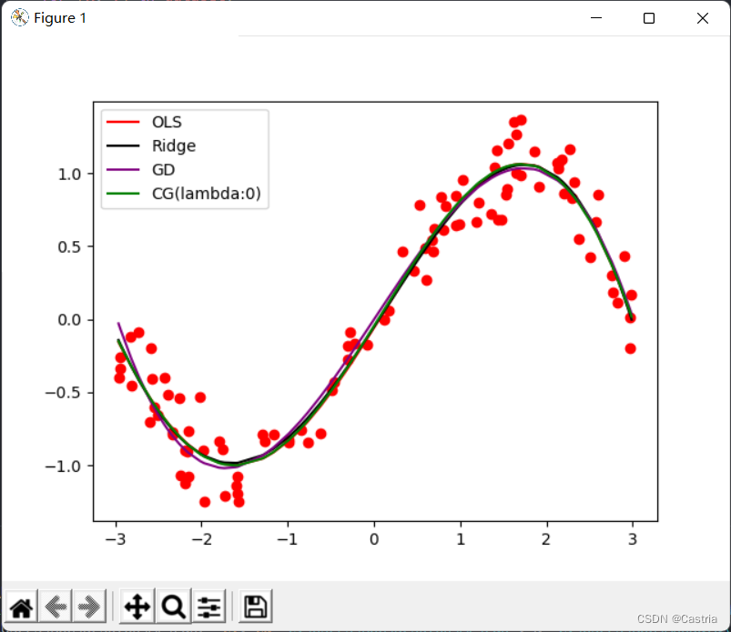
Finally, the fitting images of the four methods (basically the same) and the main function are attached, and the parameters can be adjusted according to the experimental requirements:

if __name__ == '__main__':
    warnings.simplefilter('error')

    dataset = get_dataset(bound = (-3, 3))
    # 绘制数据集散点图
    for [x, y] in dataset:
        plt.scatter(x, y, color = 'red')
    
    
    # 最小二乘法
    coef1 = fit(dataset)
    # 岭回归
    coef2 = ridge_regression(dataset)
    # 梯度下降法
    coef3 = GD(dataset, m = 3)
    # 共轭梯度法
    coef4 = CG(dataset)
    
    # 绘制出四种方法的曲线
    draw(dataset, coef1, color = 'red', label = 'OLS')
    draw(dataset, coef2, color = 'black', label = 'Ridge')
    draw(dataset, coef3, color = 'purple', label = 'GD')
    draw(dataset, coef4, color = 'green', label = 'CG(lambda:0)')

    # 绘制标签, 显示图像
    plt.legend()
    plt.show()