4.1 How to effectively optimize the model
4.1.1 Optimization from business ideas
1) Are there more obvious and intuitive rules and indicators that can replace complex modeling?
2) Are there any obvious business logics (business assumptions) that were overlooked in the early modeling stage?
3) Through preliminary modeling and data familiarization, are there any new discoveries that can even subvert previous business speculation (intuition)?
4) Is the definition of the target variable stable (validated by sampling at different time points)?
4.1.2 Optimization from the technical idea of modeling
1) Comparison of different modeling algorithms
2) Comparison of different sampling methods
3) Is it necessary to model separately by subdividing groups?
4.2 The main index system of model effect evaluation
This section will focus on evaluation metrics for classification (prediction) models where the target variable is a binary variable
4.2.1 A series of indicators to evaluate the accuracy and precision of the model
First define the following four basic definitions:
|
|
predicted class |
||
|
|
1 |
0 |
|
| actual category |
1 |
TP |
FN |
| 0 |
FP |
TN |
|
From this, the following evaluation indicators are extended
1) Correct rate: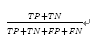
2) Error rate:
3) Sensitivity:
4) Special effect:
5) Accuracy:
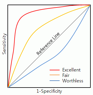
4.2.2 ROC curve
The ROC curve is a visual tool for effectively comparing two binary classification models, showing a comparative rating between true and false positive rates of sensitivity for a given model. The increase of the true rate is at the expense of the increase of the false positive rate. The area under the ROC curve is the index and basis for comparing the accuracy of the model. The model with a larger area has a higher model accuracy, that is, the model that needs to be selected for application. The closer the area is to 0.5, the lower the accuracy of the corresponding model.
To draw the ROC curve, first of all, the judgments made by the model, that is, the data, are sorted, and the probability that the observed values after judgment by the model are predicted to be positive (1) is sorted from high to low. The vertical axis of the ROC curve represents the true rate, and the horizontal axis of the ROC curve represents the false positive rate. When drawing specifically, starting from the lower left corner, the true rate and false positive rate are both 0. According to the order of probability from high to low, draw the actual "positive" or "negative" of each observation value in turn, if it is is truly "positive" (predicted correctly), the ROC curve moves up and draws a point; if it is truly "negative", the ROC curve moves one point to the right.
4.2.3 KS value
The larger the value of KS, the greater the ability of the model to distinguish positive (1) and negative (0) customers, and the higher the accuracy of the model prediction. Generally speaking, KS greater than 0.2 indicates that the model has better prediction accuracy.
The steps to draw the KS curve are as follows:
1) Rank all the observed objects in the test set that are predicted to be positive (1) by the model scoring in descending order of probability.
2) Calculate the cumulative value of the observed objects that are actually positive (1) and negative (0) corresponding to each probability score, and the total number of the total number of positive (1) and negative (0) that they account for respectively. percentage.
3) Plot the two cumulative percentages and scoring points on the same graph to get the KS curve, as shown below:
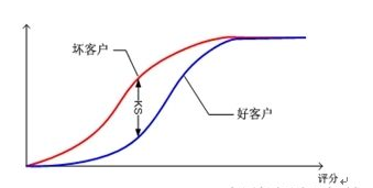
4) The maximum value of the difference between the cumulative percentage of true positive (1) observations and the cumulative percentage of true negative (0) observations under each score is the KS value.
4.2.4 lift value
We know that the binary prediction model has a random rate in specific business scenarios. The so-called random rate refers to the positive proportion based on the existing business effect when the model is not used, that is, it is "positive" before the model is not used. The proportion of actual observed objects in the total observed objects. If there is a good model after modeling, then this model can effectively lock the group. The so-called effective means that in the ranking of the predicted probability values from high to low, among the top observations, the true The proportion of "positive" observations in the cumulative total observations should be higher than the random rate.

From the above lift formula, two evaluation indicators commonly used in model evaluation are derived, namely the response rate (%response) and the capture rate (%captured response). First, the observation objects that are predicted by the model to be positive (1) are sorted according to the predicted probability from high to low, and then these observation objects are divided into 10 intervals according to the equal number, and the number of observation objects in each interval is the same, so that Individual intervals may be named Top 10% of Objects, Top 20% of Objects, and so on.
Response rate refers to the percentage of observation objects that actually belong to positive (1) in a certain interval or cumulative interval observation objects sorted by the above probability scores to the total number of observation objects in this interval or in this cumulative interval. Obviously, the higher the response rate, the higher the prediction accuracy of the interval.
The capture rate refers to the percentage of observation objects that actually belong to positive (1) in the total number of observation objects that belong to positive (1) among the observation objects in the above ranking interval, and the higher the better.