Detailed explanation of the underlying execution process of Spark SQL

Contents of this article
1. Apache Spark
2. The development
of Spark SQL 3. The underlying execution principle of Spark SQL
4. Two optimizations of Catalyst

The full version of Portal: Spark Knowledge System nanny-level summary, 50,000 words of good text!

1. Apache Spark

Apache Spark is a unified analysis engine for large-scale data processing . Based on in- memory computing , it improves the real-time performance of data processing in a big data environment, while ensuring high fault tolerance and scalability , allowing users to deploy Spark in a large number of On top of the hardware, a cluster is formed.

Spark source code has grown from 40w lines in 1.x to more than 100w lines now, and more than 1400 big cows have contributed code. The entire Spark framework source code is a huge project.

Second, the development history of Spark SQL

We know that Hive implements SQL on Hadoop, which simplifies MapReduce tasks and can perform large-scale data processing only by writing SQL, but Hive also has a fatal disadvantage, because the bottom layer uses MapReduce for computing, and the query latency is high.

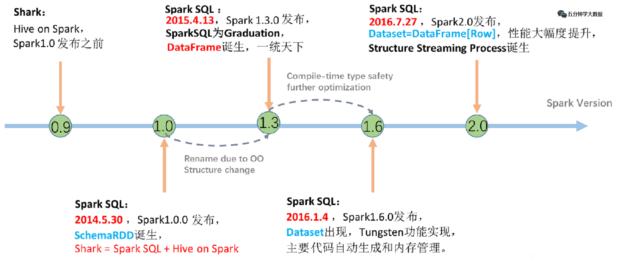
1. The Birth of Shark

So Spark launched Shark in the early version (before 1.0) , what is this? Shark and Hive are actually closely related. Many things at the bottom of Shark still depend on Hive, but modified memory management, physical plan, execution three Module, the bottom layer uses Spark's memory-based computing model, which improves the performance several times to hundreds of times compared to Hive.

The problem arises:

1. Because the generation of Shark execution plan relies heavily on Hive, it is very difficult to add new optimizations;

2. Hive is process-level parallelism, and Spark is thread-level parallelism, so many thread-unsafe codes in Hive are not suitable for Spark;

3. Due to the above problems, Shark maintains a branch of Hive, and it cannot be merged into the main line, making it difficult to sustain;

4. At the Spark Summit on July 1, 2014, Databricks announced the end of development of Shark, focusing on Spark SQL.

2. SparkSQL-DataFrame was born

Solve the problem:

1. Spark SQL execution plan and optimization are handed over to the optimizer Catalyst;

2. A set of simple SQL parser is built-in, and HQL is not required;

3. It also introduces DSL APIs such as DataFrame, which can be completely independent of any Hive components.

New question :

For the initial version of SparkSQL, there are still many problems, such as it can only support the use of SQL, cannot be well compatible with the imperative format, and the entry is not unified enough.

3. SparkSQL-Dataset was born

In the 1.6 era, SparkSQL added a new API called Dataset. Dataset unifies and combines the use of SQL access and imperative API, which is an epoch-making progress.

In Dataset, you can easily query and filter data using SQL, and then perform exploratory analysis using the imperative API.

3. The underlying execution principle of Spark SQL

The underlying architecture of Spark SQL is roughly as follows:

As you can see, the SQL statements we wrote are converted into RDDs by an optimizer (Catalyst) and handed over to the cluster for execution.

There is a Catalyst between SQL and RDD, which is the core of Spark SQL. It is a query optimization framework for the execution of Spark SQL statements, based on the Scala functional programming structure.

If we want to understand the execution process of Spark SQL, it is very necessary to understand the workflow of Catalyst.

An SQL statement generates a program that can be recognized by the execution engine, and it is inseparable from the three processes of parsing (Parser), optimization (Optimizer), and execution (Execution) . When the Catalyst optimizer performs plan generation and optimization , it is inseparable from its own internal five components, as follows:

1. Parser module : parses SparkSql strings into an abstract syntax tree/AST.

2. Analyzer module : This module traverses the entire AST, binds data types and functions to each node on the AST, and then parses the fields in the data table according to the metadata information Catalog.

3. Optimizer module : This module is the core of Catalyst. It is mainly divided into two optimization strategies, RBO and CBO. RBO is rule-based optimization, and CBO is cost-based optimization .

4. SparkPlanner module : The optimized logical execution plan OptimizedLogicalPlan is still logical and cannot be understood by the Spark system. At this time, the OptimizedLogicalPlan needs to be converted into a physical plan .

5. CostModel module : Choose the best physical execution plan mainly based on past performance statistics. The optimization of this process is CBO (cost-based optimization).

In order to better understand the whole process, the following simple examples are explained.

Step 1. Parser Phase: Unparsed Logical Plan

Parser simply means that the SQL string is divided into tokens one by one, and then parsed into a syntax tree according to certain semantic rules. The Parser module is currently implemented using the third-party class library ANTLR , including the familiar Hive, Presto, SparkSQL, etc., which are all implemented by ANTLR .

In this process, it will be judged whether the SQL statement conforms to the specification, such as whether the keywords such as select from where are written correctly. Of course, table names and table fields will not be checked at this stage.

Step 2. Analyzer Phase: Parsed Logical Plan

The parsed logical plan basically has a skeleton. At this time, basic metadata information is required to express these morphemes. The most important metadata information mainly includes two parts: the Scheme of the table and the basic function information . The Scheme of the table mainly includes the table's scheme. Basic definition (column name, data type), table data format (Json, Text), table physical location, etc. Basic functions mainly refer to class information.

ageAnalyzer will traverse the entire syntax tree again, and perform data type binding and function binding on each node on the tree. For example, the people morpheme will be parsed into a table containing and three columns according to the metadata table information , idwhich will be parsed as a data type . A variable of , which is resolved to a specific aggregate function.namepeople.ageintsum

This process will determine whether the table name and field name of the SQL statement really exist in the metadata database.

Step 3. Optimizer Module: Optimized Logical Plan

The Optimizer optimization module is the core of the entire Catalyst. As mentioned above, the optimizer is divided into two types: rule-based optimization (RBO) and cost-based optimization (CBO). The rule-based optimization strategy is actually a traversal of the syntax tree, and the pattern matching is performed on nodes that satisfy a specific rule, and the corresponding equivalent transformation is performed. Three common rules are described below: Predicate Pushdown , Constant Folding , and Column Pruning .

• Predicate Pushdown

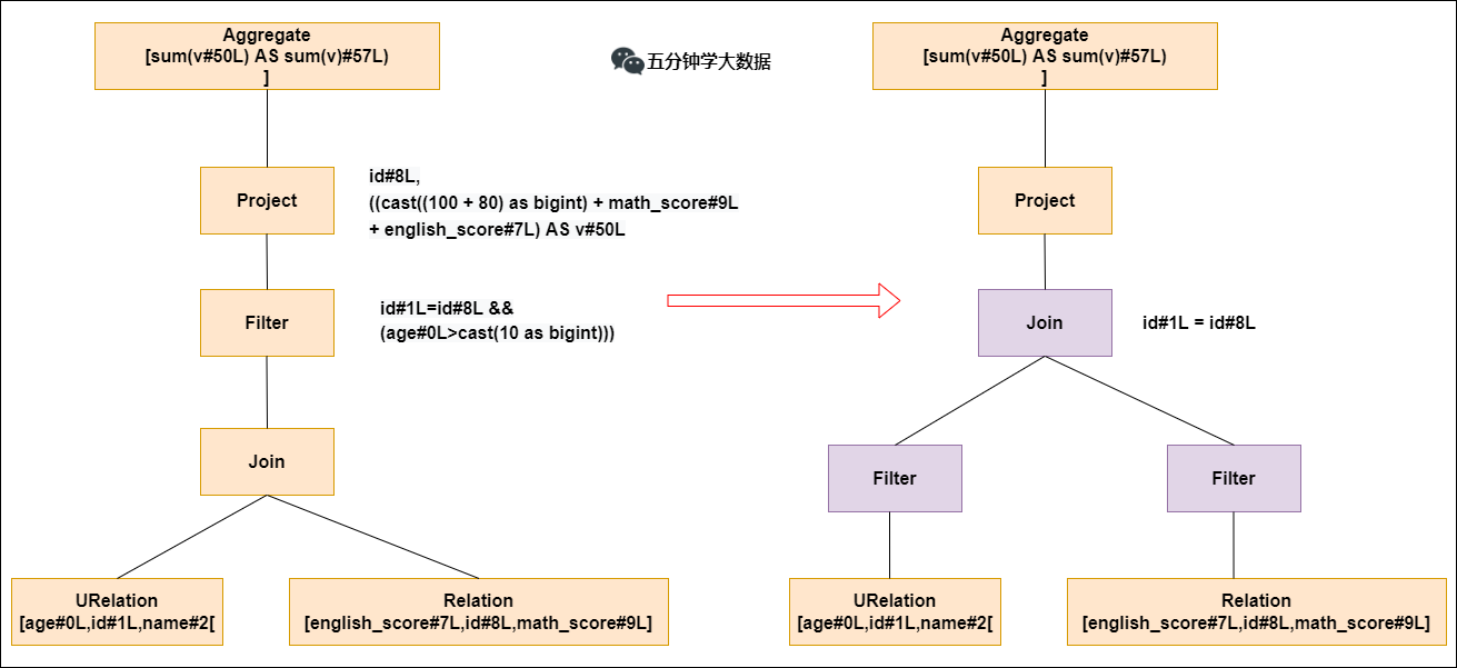
The left side of the above figure is the parsed syntax tree. The two tables in the syntax tree are done first join, and then the age>10filter is used. The join operator is a very time-consuming operator. The time-consuming operation generally depends on the size of the two tables involved in the join. If the size of the two tables involved in the join can be reduced, the time required for the join operator can be greatly reduced.

Predicate pushdown is to push down the filtering operation before join, and when join is performed later, the amount of data will be significantly reduced, and the join time will inevitably be reduced.

• Constant Folding

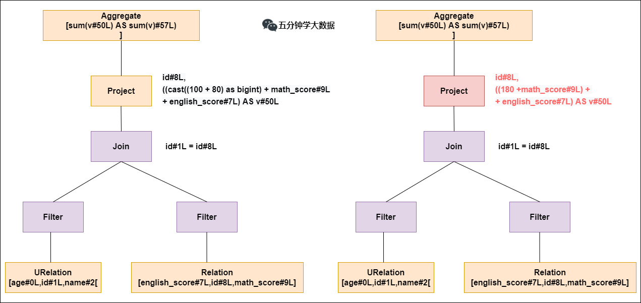
Constant accumulation is such as calculation x+(100+80)->x+180, although it is a small change, but it is of great significance. Without optimization, each result would need to be performed once 100+80and then added to the result. After optimization, there is no need to perform the 100+80operation again.

• Column Pruning

Column value clipping is that when a table is used, it does not need to scan all its column values, but scans only the ids that are needed, and clips those that are not needed. On the one hand, this optimization greatly reduces the consumption of network and memory data, and on the other hand, it greatly improves the scanning efficiency for columnar storage databases.

Step 4. SparkPlanner Module: Convert to Physical Execution Plan

According to the above steps, the logical execution plan has been optimized. However, the logical execution plan still cannot be executed. They are only logically feasible. In fact, Spark does not know how to execute this thing. For example, join is an abstract concept, which means that two tables are merged according to the same id. However, the logic execution plan does not explain how to implement the merge.

At this point, it is necessary to convert the logical execution plan into a physical execution plan, that is, to change the logically feasible execution plan into a plan that Spark can actually execute. For example, for the join operator, Spark formulates different algorithm strategies for the operator according to different scenarios. There are BroadcastHashJoin, ShuffleHashJoinand SortMergejoinso on. The physical execution plan is actually to select an algorithm implementation with the least time-consuming among these specific implementations. How to choose, the following is simple Say:

• In fact, SparkPlanner converts the optimized logical plan to generate multiple physical plans that can be executed ;

• Then the CBO (cost-based optimization) optimization strategy will calculate the cost of each Physical Plan according to the Cost Model , and select the Physical Plan with the smallest cost as the final Physical Plan.

The above steps 2, 3, and 4 are combined, which is the Catalyst optimizer!

Step 5. Execute the physical plan

Finally, according to the optimal physical execution plan, generate java bytecode, convert SQL into DAG, and operate in the form of RDD.

Summary: Overall Execution Flowchart

4. Two optimizations of Catalyst

Here we summarize two important optimizations of the Catalyst optimizer.

1. RBO: Rule-Based Optimization

Optimization points such as: predicate pushdown, column clipping, constant accumulation, etc.

• Predicate pushdown case :

select 
* 
from 
table1 a 
join 
table2 b 
on a.id=b.id 
where a.age>20 and b.cid=1

The above statement is automatically optimized to look like this:

select 
*
from
(select * from table1 where age>20) a
join
(select * from table2 where cid=1) b
on a.id=b.id 

That is, the data is filtered in advance in the sub-query stage, and the amount of shuffled data in the later join is greatly reduced.

• Column clipping case :

select
a.name, a.age, b.cid
from
(select * from table1 where age>20) a
join
(select * from table2 where cid=1) b
on a.id=b.id

The above statement is automatically optimized to look like this:

select 
a.name, a.age, b.cid
from
(select name, age, id from table1 where age>20) a
join
(select id, cid from table2 where cid=1) b
on a.id=b.id

It is to query the required columns in advance, and cut out other unnecessary columns.

• Constant accumulation :

select 1+1 as id from table1

The above statement is automatically optimized to look like this:

select 2 as id from table1

That is, it will be 1+1calculated in advance 2, and then assigned to each row of the id column, without calculating it every time 1+1.

2. CBO: Cost-Based Optimization

That is, after SparkPlanner generates multiple executable physical plans for the optimized logical plan, the multiple physical execution plans select the optimal physical plan with the least execution time based on the Cost Model .

reference:

Spark knowledge system nanny-level summary, 50,000 words of good text!

{{o.name}}

{{m.name}}