Article directory
Graphical and textual explanation of PID parameter tuning
After reading this article, you will gain:
- Basic concept of three parameters of PID
- Learn how to tune PID
- Get to know a blogger who's always googling
First on the renderings:
1. What is PID
In engineering, if we want to use a single-chip microcomputer to make a temperature control system, the system composition is generally as follows: an ADC for collecting temperature, a heating head for outputting temperature, and a single-chip microcomputer for running the control algorithm. If we want to maintain the temperature as 100 degrees, without adding any control algorithm, we can control the temperature through a simple threshold judgment method , an if judgment statement, when the collected temperature is greater than 100, the microcontroller controls the heating head to turn off, when the collected temperature is less than At 100 degrees, the single-chip microcomputer controls the heating head to turn on, which is simple and rude, but the temperature curve displayed by such a control method is extremely unstable. As a result, the final temperature curve will oscillate around the target, which cannot achieve the desired control effect, as shown in the figure below: the actual curve (black line) oscillates around the target curve (red line)
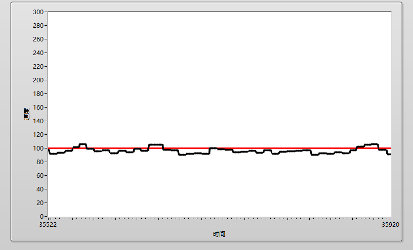
So how can we maintain the actual curve to fit the target curve and achieve a stable control effect?
The concept of PID control algorithm is introduced here. PID is the abbreviation of Proportion Integration Differentiation . In fact, it is a formula, which consists of three parts: Proportion , Integration and Differentiation . , the specific form is the following formula:
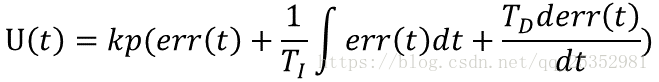
Among them, err(t) is the error between the current value and the target value. The formula of PID is to perform proportional, integral and differential processing on this error and then superimpose the output . Because the calculation definitions of proportional calculation, integral calculation and differential calculation are different in mathematical formulas , so the output characteristics and input characteristics of the corresponding items are also different. The specific explanation is as follows:
1. Scale factor
The proportional control coefficient is actually a simple definition of the linear relationship between input and output. If the value range of our output control quantity is 100-1000, the input err error range is 0.001-0.1; when the error is 0.1, the output quantity Need to reach 1000, then we need to build a linear relationship between input and output through the proportional coefficient
2. Integral factor
In the previous point, we analyzed the meaning of the proportional coefficient. Some friends may be curious. The effect of adding the proportional coefficient is actually no different from the threshold judgment principle. It is indeed the case. The effect of only using the proportional coefficient is no different from the threshold judgment, but Don't forget, there are two items of I and D behind PID. The understanding of the I item can be understood from the meaning of integral. Integral can be understood as the area of the curve enclosed by curves, straight lines and axes on the coordinate plane. value, this curve is the function of err(t), and the integral area value is the accumulated error value representing the past period of time. We multiply this accumulated value by the coefficient to transform and superimpose it on the output, which can eliminate the history to a certain extent. The influence of the error on the current actual curve to improve the stability of the system
3. Differential coefficient
The mathematical understanding of differential can be understood as the slope of the current error curve. It can be used to predict the future trend of the current curve. After processing the value of the differential term and superimposing it, the future trend of the current value can be predicted and the system can be used to improve the ability to respond to future changes.
2. PID adjustment method
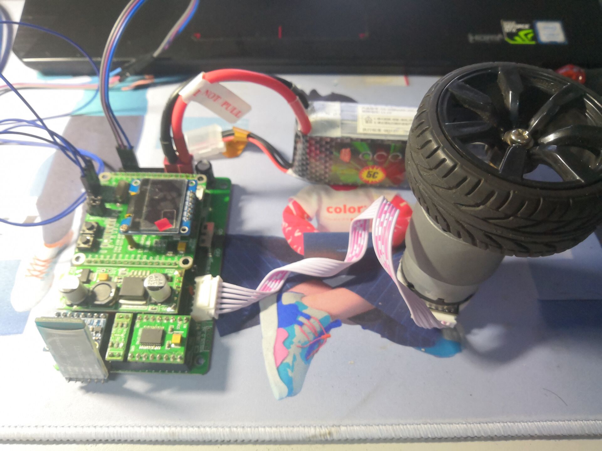
Through the analysis in the previous section, we have a simple understanding of the three items of PID, but the description in the text is still too abstract. I will use a car speed control system for further explanation, and analyze the three PID three items in combination with the actual phenomenon. The actual function of these three parameters, and how to adjust these three parameters, the experimental platform used is as follows
-
The main control board and motor of the balance car home
-
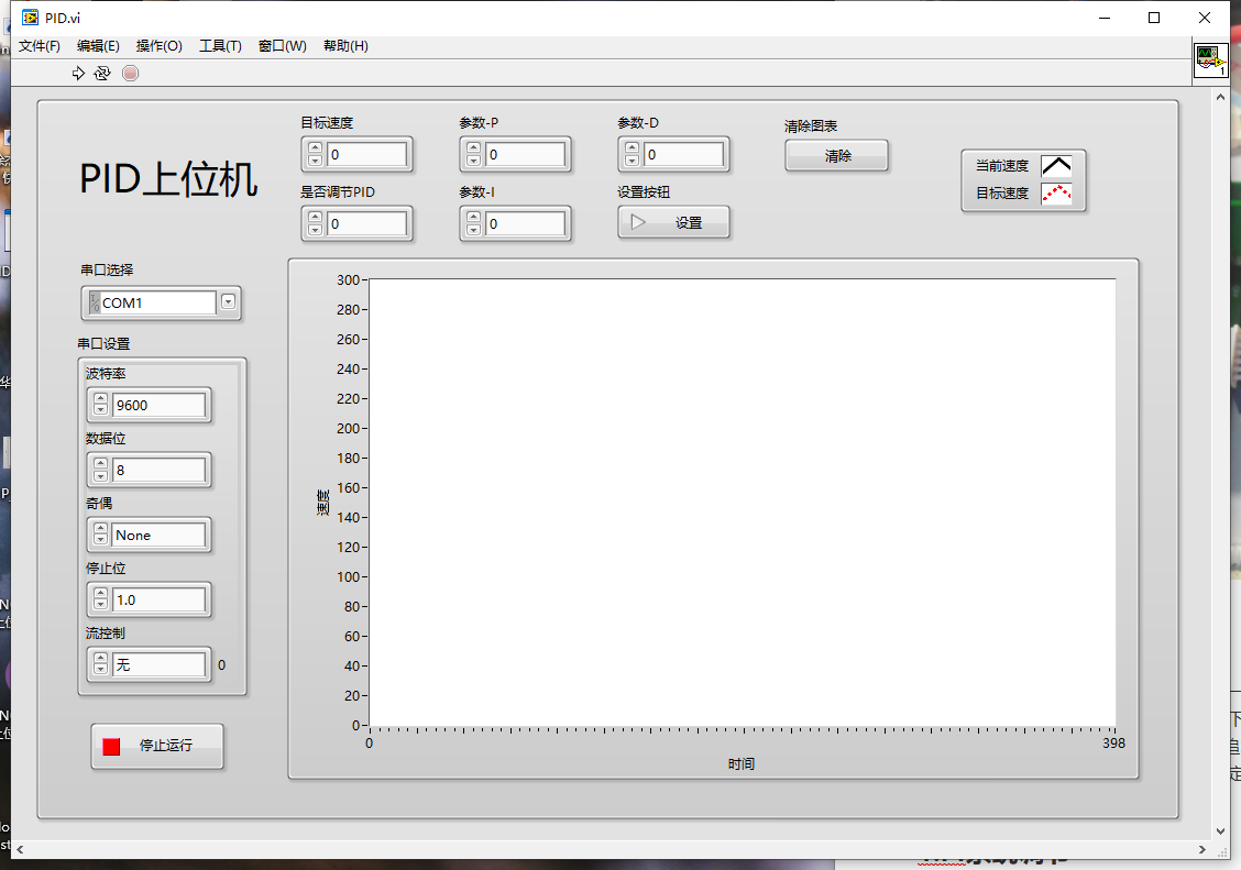
Self-written debugging host computer
Control system picture:
Host computer interface:
When we use PID, it is meaningless to use only one parameter alone. At least two parameters are used , and P (proportional term) is necessary. Although PID has three parameters, in most cases PID has three parameters Not all of them are used. Generally, two of them are used in combination. For example, the PI combination is used for a stable system, and the PD combination is used for a fast response system. Of course, PID is used for both stable and fast response systems. But in fact, the more PID parameters, the more difficult it is to adjust, and in many cases the effect of two parameters is enough, so I generally use the first two according to the situation, and the following is an analysis of these systems.
1. PI system adjustment
The first step in adjusting the PI system is to adjust P first, from small to large. The value of P can be clearly reflected in the output curve. For example, if I give P=0.05 first, the system responds as follows. When P is too small, the curve will Shows a slow rise , and the final value will be significantly lower than the target value
When we increase P to 0.15, we can see that the actual curve is very close to the target value, but because there is only pure P control, there is a large overshoot (overshoot is that the actual value cannot stop the car when it reaches the target value) , rushed out) , but when he stabilized, the actual curve was basically close to the target curve

If P is increased to 0.25, it can be seen that the actual curve needs to oscillate for a long time to reach the stable target line , but after stabilization, it is basically consistent with the target line

If P is too large, the whole system will be out of control, the actual curve will not converge to the target curve position, and there will be constant amplitude oscillation , such as when P=0.45

When adjusting the PI system, there are generally two cases for the selection of P
-
P is a little smaller. When stable, the actual value is below the target value, and there is always an error. At this time, start from 0 and increase I all the time to eliminate the error during stability. In this case, the final stability curve will always remain at Below the target curve, a relatively stable adjustment effect is achieved, and there will be no overshoot
(No overshoot, stable!)
-
When P is larger, there is a certain overshoot when the target value is reached for the first time, but it will stabilize after that, and its response speed is faster than the first one!
(There is overshoot, but he is fast!)
The first PI control method is shown below. When P=0.5 (smaller), I can be used to eliminate the steady-state error during stability to achieve a stable effect:
The value of I integral here I show three, respectively, the actual curve when it is smaller, just right, and larger, for comparison!
P=0.5, I=0.00005, I select a small value, it can be seen that compared with the simple P=0.5, the stability error has been eliminated to a certain extent, but the degree of elimination is not enough!
When increasing I to 0.0001, just right, the actual curve and the target curve basically coincide! ! !

When I is too large to take 0.002, because the cumulative error proportion is too large, there will be jitter and it is difficult to converge
The above is the first PI adjustment situation. Although the balance process of the PI system is very stable, the response speed to the target position is slow . P=0.07, when the corresponding I is 0.0001, the waveform is as follows. The system allows a certain overshoot, but it can reach the target point faster and then stabilize. This is the second adjustment method of the PI system.

The above is basically the adjustment process of the PI system. Let me talk about the adjustment process of the PD system.
2. PD system adjustment
From the concept at the beginning, we can know that the difference from I is that I calculates the cumulative error, and D calculates the future trend, so the PD system has a faster response speed and will reach the target position faster than the PI system. Nearby, its adjustment method is to adjust P first . Here we adjust P to a larger position according to the adjustment result of P in PI, and there is a certain overshoot. Here we take P=0.15, and the graph is as follows when D is not added:

It can be seen from the image: P=0.15 has serious overshoot at the beginning, so add a D to reduce the overshoot amplitude. The selection of D is the same as the selection of I, and it gradually increases from 0. The viewing effect determines the appropriate point. D=1.5 in the picture below is a more suitable point for me to try out. We can see that after adding a suitable D, the actual curve reaches the target position in a shorter time, and the overshoot amplitude is also reduced , but the effect here is not Obviously, the main reason is that the speed PID I use here is the small wheel, and the application of PD is mainly in the large inertia system. The application scene here is not suitable, but it can also be seen to some extent.

If D is adjusted too large, it will amplify the influence of the system trend, causing the system to oscillate and be difficult to stabilize, as follows: D=5
3. PID system adjustment
After talking about the adjustment methods of the PI and PD systems, let's share the adjustment methods of the PID system. First, we first adjust according to the PI system, first adjust the P and then adjust the I, so that the system can stabilize after a certain overshoot , as shown in the following figure :

After the above PI waveform appears, start to adjust D below , slowly increase D, and compensate for the overshoot until the system is stable. The final effect is as shown in the figure below, and the PID system is basically adjusted.
The PID explanation of this article is here. The next article will share the PID calling code I often use in detail to help you get started with PID. The
second article has been updated, article link: write a PID control code from 0
Irons! If you find it useful, just click three times!
Recommended articles in the past
The 200 yuan development board runs the neural network model and hangs OpenMV!
GD32 replaces STM32 whole process record
51 single-chip multi-threading artifact: Tiny-51 operating system
High-precision temperature measurement and control system based on STM32 - schematic design