
Python has become one of the most popular languages in the field of data science in recent years. One of the important reasons is that Python has a large number of easy-to-use packages and tools. Among these libraries, Pandas is one of the most practical tools for data science operations. This article shares 12 Pandas methods for Python data manipulation, and also adds some tips and suggestions that can improve your work efficiency.
Data set: This article uses the data set used in a "loan prediction" problem in the Analytics Vidhya data science competition.
https://datahack.analyticsvidhya.com/contest/practice-problem-loan-prediction-iii/
First, we import the module and load the dataset into the Python environment:
import pandas as pd
import numpy as np
data = pd.read_csv("train.csv", index_col="Loan_ID")
Boolean index
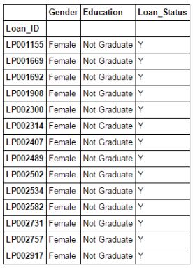
What if you want to filter out the value of a column from a set of columns based on certain conditions? For example, we want a list that contains a list of all women who have taken out loans and have not yet graduated. Using Boolean indexing here can help. You can use the following code:
data.loc[(data["Gender"]=="Female") & (data["Education"]=="Not Graduate") & (data["Loan_Status"]=="Y"), ["Gender","Education","Loan_Status"]]
Apply function
The Apply function is one of the commonly used functions for processing data and creating new variables. After applying a function to a row/column of the DataFrame, Apply returns some values. The function can either use the default or customize it. For example, it can be used here to find missing values for each row and each column.
#创建一个新函数
def num_missing(x):
return sum(x.isnull())
#应用每一列
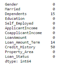
print "Missing values per column:"
print data.apply(num_missing, axis=0) #axis=0 defines that function is to be applied on each column
#应用每一行
print "\nMissing values per row:"
print data.apply(num_missing, axis=1).head() #axis=1 defines that function is to be applied on each row
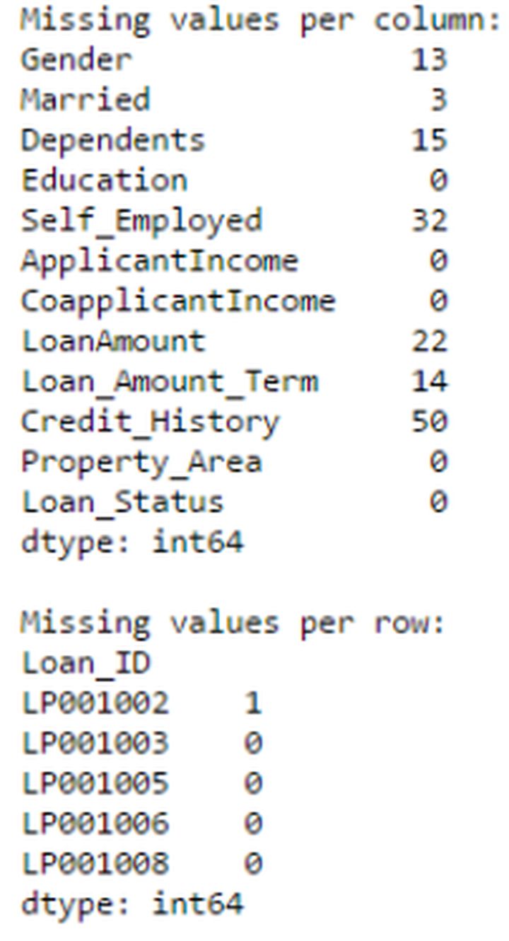
In this way we got the desired result.
Note: Use the head() function in the second output because it contains many lines.
Replace missing values
Use fillna() to replace missing values in one step. It can update missing values with the average/mode/median of the target column. In the following example, we use the modes of the columns'Gender','Married' and'Self_Employed' to replace their missing values.
#首先我们导入一个函数来确定模式
from scipy.stats import mode
mode(data['Gender'])
Output:
ModeResult(mode=array([‘Male’], dtype=object), count=array([489]))
Remember, the mode is sometimes an array because there may be multiple high-frequency values. By default we use the first one:
mode(data['Gender']).mode[0]Output:
‘Male’Now we can fill in the missing values, use the second method above to check.
#导入值:
data['Gender'].fillna(mode(data['Gender']).mode[0], inplace=True)
data['Married'].fillna(mode(data['Married']).mode[0], inplace=True)
data['Self_Employed'].fillna(mode(data['Self_Employed']).mode[0], inplace=True)

#现在再次检查缺失值进行确认:
print data.apply(num_missing, axis=0)
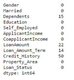
It is confirmed that the missing value has been replaced. Note that this is just a common replacement method, and there are other complex methods, such as modeling missing values.
Pivot table
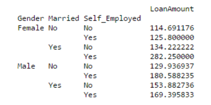
Pandas can also be used to create Excel-style pivot tables. For example, in our example, the key column of the data is'LoanAmount' which contains missing values. We can replace the missing values with the average of the groups'Gender','Married' and'Self_Employed'. In this way, the average'LoanAmount' of each group can be determined as:
#确定数据透视表
impute_grps = data.pivot_table(values=["LoanAmount"], index=["Gender","Married","Self_Employed"], aggfunc=np.mean)
print impute_grps
Multiple index
If you pay attention to the output of the third technique, you will find that it has a strange feature: each index consists of 3 values. This is multi-index, it can speed up our operation speed.
Continuing with the example of the third technique above, we have values for each group, but we have not yet estimated the missing values.
We can use the techniques we used before to solve this problem:
#用缺失的 LoanAmount仅迭代所有的行
for i,row in data.loc[data['LoanAmount'].isnull(),:].iterrows():
  ind = tuple([row['Gender'],row['Married'],row['Self_Employed']])
  data.loc[i,'LoanAmount'] = impute_grps.loc[ind].values[0]

#现在再次检查缺失值进行确认
print data.apply(num_missing, axis=0)
note:
Multi-index requires a tuple to define the index group in the loc statement, which is a tuple used in the function.
The .values[0] suffix here is necessary because by default a series of elements will be returned, which will produce an index that does not match the DataFrame. In this example, assigning values directly will produce an error.
Crosstab
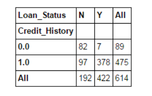
This function is used to obtain a preliminary "feel" (overview) of the data. Here, we can verify a basic assumption. For example, in this example, we expect that "Credit_History" will greatly affect the loan status. Then we can use the cross table as shown below to test:
pd.crosstab(data["Credit_History"],data["Loan_Status"],margins=True)
These are absolute values. However, it is more intuitive to use percentages. We can use the apply function to complete:
def percConvert(ser):
  return ser/float(ser[-1])
  pd.crosstab(data["Credit_History"],data["Loan_Status"],margins=True).apply(percConvert, axis=1)
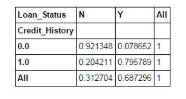
Now, it is clear that people with a credit history have a higher chance of obtaining a loan: 80%, compared with 9% for people without credit.
But the fact is not so simple. Since we know that having a credit history is very important, what if we predict the borrowing status of a person with a credit history as Y and a person without a credit history as N? We will be surprised to find that out of all 614 tests, 82+378=460 predictions were correct, and the accuracy rate reached 75%!
You may wonder why we need statistical models, but you have to know that it is a very difficult challenge to increase the accuracy even by 0.001%.
Note: The 75% accuracy rate is the accuracy rate obtained on the training set. It will be slightly different on the test set, but it is similar.
Merge DataFrame
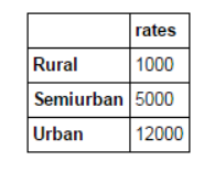
If we have information from multiple data sources that need to be checked, then merging DataFrame will be a basic operation. Consider a hypothetical situation where different property types have different average property prices (prices per square meter). We define the DataFrame as:
prop_rates = pd.DataFrame([1000, 5000, 12000], index=['Rural','Semiurban','Urban'],columns=['rates'])
prop_rates
Now, we can merge this information with the initial DataFrame into:
data_merged = data.merge(right=prop_rates, how='inner',left_on='Property_Area',right_index=True, sort=False)
data_merged.pivot_table(values='Credit_History',index=['Property_Area','rates'], aggfunc=len)
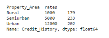
Through the pivot table, we can know that the merge was successful. Note that the'values' parameter has nothing to do with this, because we just simply calculate the value.
Sort DataFrame
Pandas allows us to sort by multiple columns easily, which can be done as follows:
data_sorted = data.sort_values(['ApplicantIncome','CoapplicantIncome'], ascending=False)
data_sorted[['ApplicantIncome','CoapplicantIncome']].head(10)
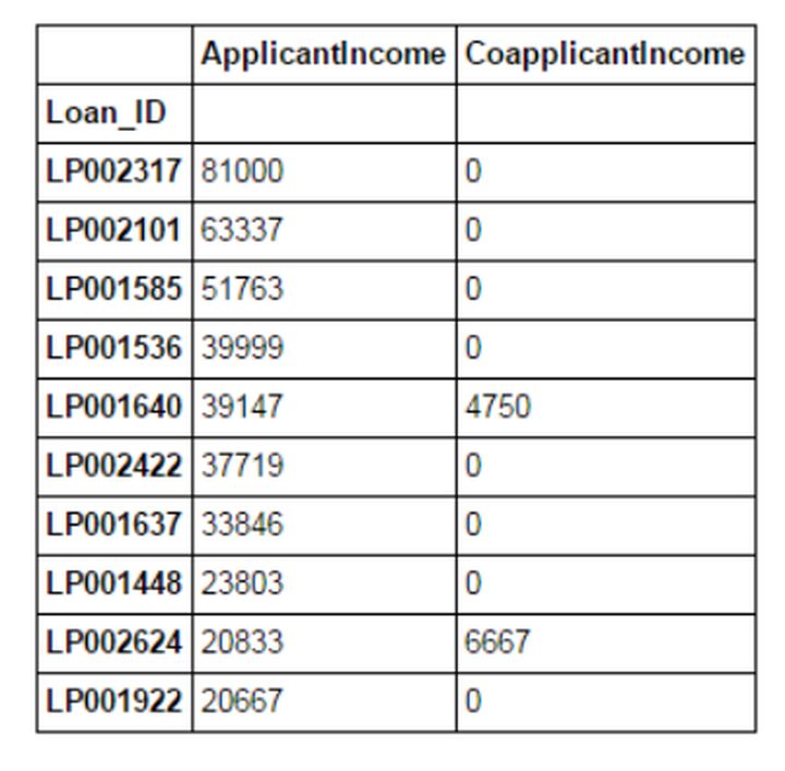
Note: The "Sort" function of Pandas is no longer available, we should use "sort_values" instead.
Plotting (box plot & histogram)
Many people may not know that we can draw box plots and histograms directly on Pandas. In fact, there is no need to call matplotlib. Only one line of command is required. For example, if we want to compare the income distribution of loan applicants based on Loan_Status:
import matplotlib.pyplot as plt
%matplotlib inline
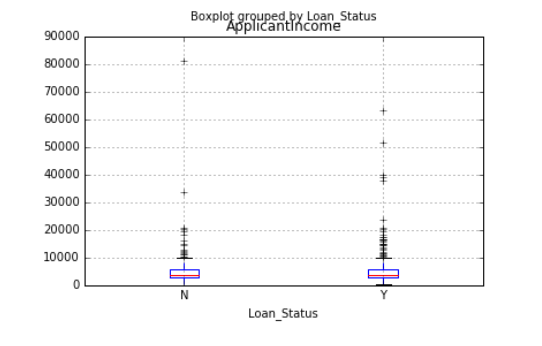
data.boxplot(column="ApplicantIncome",by="Loan_Status")
data.hist(column="ApplicantIncome",by="Loan_Status",bins=30)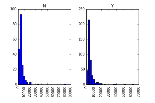
As you can see from the chart, income is not a big decisive factor, because there is no obvious difference between the income of the person who received the loan and the person who was denied the loan.
Use cut function for data combination
Sometimes after clustering, the value will be more meaningful. For example, we want to model the traffic flow in a day (the time unit is minutes), accurate to every hour and every minute. For predicting the traffic flow, the correlation may not be so high. Use the actual time period of the day such as "morning "Afternoon", "Evening", "Night" and "Late night" will have better effects. Modeling the traffic flow in this way will be more intuitive and avoid overfitting.
Here we define a simple function that can be reused to combine any variables:
#组合:
def binning(col, cut_points, labels=None):
#定义最小和最大值
minval = col.min()
maxval = col.max()
#向cut_points添加最大和最小值来创建列表
break_points = [minval] + cut_points + [maxval]
#如果没提供标签就用默认标签 0 ... (n-1)
if not labels:
labels = range(len(cut_points)+1)
#用Pandas的cut函数进行组合
colBin = pd.cut(col,bins=break_points,labels=labels,include_lowest=True)
return colBin
#组合:
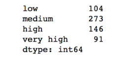
cut_points = [90,140,190]
labels = ["low","medium","high","very high"]
data["LoanAmount_Bin"] = binning(data["LoanAmount"], cut_points, labels)
print pd.value_counts(data["LoanAmount_Bin"], sort=False)
Code name data
Usually we will encounter a situation where the category of the nominal variable must be modified. This may be due to several reasons:
Some algorithms (such as logistic regression) require all inputs to be numeric. Therefore, most nominal variables are written as 0,1···(n-1).
Sometimes a category can be expressed in two ways. For example, the temperature can be recorded as "High", "Medium" and "Low", or "H" and "low", where both "High" and "H" indicate the same category. Similarly, "Low" and "low" are only slightly different. However, Python will read them as different levels.
Some categories may appear very low, so it is usually a good idea to merge them. Here we define a general function whose input is in the form of a dictionary, and then use the'replace' function in Pandas to encode the input value.
#用Pandas的replace函数定义一个通用函数
def coding(col, codeDict):
colCoded = pd.Series(col, copy=True)
for key, value in codeDict.items():
colCoded.replace(key, value, inplace=True)
return colCoded
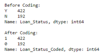
#将LoanStatus 编码为 Y=1, N=0:
print 'Before Coding:'
print pd.value_counts(data["Loan_Status"])
data["Loan_Status_Coded"] = coding(data["Loan_Status"], {'N':0,'Y':1})
print '\nAfter Coding:'
print pd.value_counts(data["Loan_Status_Coded"])
Iterate the rows of DadaFrame
This technique is not often used, but in case you encounter such a problem, you are not afraid, right? In some cases, you might use a for loop to iterate through all the rows. For example, a common problem we face is that variables in Python are not treated correctly. It usually occurs in the following two situations:
- Nominal variables with numerical categories are treated as numerical variables
- When a line with characters (due to data errors) numeric variables are treated as categorical variables
Therefore, it is often a better way to manually define the type of the column. If we check the data types of all columns:
#检查当前类型:
data.dtypes
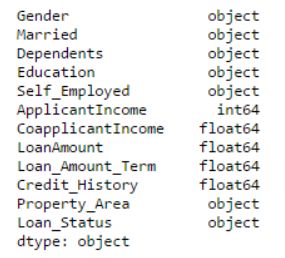
Here we can see that Credit_History is a nominal variable, but it appears as a floating point value. A good way to solve this problem is to create a CSV file with column names and types. In this way, we can write a general function to read the file and assign the column data type. For example, here we have created a CSV file datatypes.csv.
#加载文件:
colTypes = pd.read_csv('datatypes.csv')
print colTypes

After loading the file, we can iterate through each row and use the column "type" to assign the data type to the variable name defined in the "feature" column.
#迭代每一行,并分配变量类型
#注:astype 用来分配类型

for i, row in colTypes.iterrows():  #i: dataframe index; row: each row in series format
    if row['type']=="categorical":
        data[row['feature']]=data[row['feature']].astype(np.object)
    elif row['type']=="continuous":
        data[row['feature']]=data[row['feature']].astype(np.float)
print data.dtypes
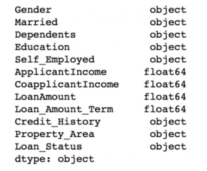
In this way, the Credit_History column is modified to an "object" type, which can be used to represent nominal variables in Pandas.
Conclusion
In this article, we explored a number of techniques in Pandas that make it more convenient and efficient for us to use Pandas to manipulate data and perform feature engineering. In addition, we have also defined some general functions, which can be reused to achieve the same effect on different data sets.