Preparation and basic principles
- Zero. Preparation and environment
- 1. Representation of digital images
- 2. Read the image
- Three. Display image
- Four. Save the picture
- Five. Data
- 6. Image type
- Seven. Image and data conversion
- 8. Array index
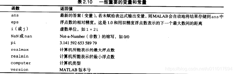
- Nine. Some important standard arrays
- 10. Operator
- 11. Flow control
- 12. Vectorization
- Thirteen.IO stream
- 14. Cell array and structure
Zero. Preparation and environment
Because I have had the basics of image processing before: PythonCV Learning Record 1-How to install the Opencv library and call
it in Python, so some details will not be recorded very detailed.
At the same time, the version of MATLAB is 2018b, which is v9.5, and I have also written an installation tutorial: Ubuntu18.04 installs Matlab2018a
Matlab use introduction does not need to be introduced. The image processing toolbox of Matlab is used in the book. I IPTfeel that the syntax is a bit like OpenCV.
Finally, the learning is based on冈萨雷斯的数字图像处理MATLAB版第三版
1. Representation of digital images
1.1 Coordinate convention
MatlabThe coordinates of is not like the way in Pythonor C++in, its origin is (1,1). And the composition of the specified tuple is (M,N) M是行 N是列.
In addition: There may be a small number of representation methods in the IPT toolbox with (row, col), please pay attention to the source code

1.2 Matrix representation
It Pythoncan be equivalent to numpyan array in the middle , and the middle C++is Mat, and I heard that it Matlabis a 面向数组的语言???so it can support array variables, and the composition is as follows:
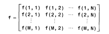
there are: 1 × Nthe matrix is a row vector, M × 1the matrix is a column vector, and 1 × 1the matrix is in 标量
Matlab The variable starts with a letter and can only consist of letters, numbers and underscores.
2. Read the image
MatlabSupports reading images in the following formats: the
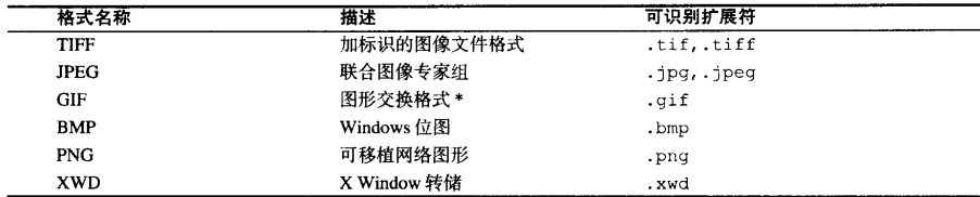
syntax is similar to CV:
f = imread('filename');
It can be an absolute path or a relative path.
Remember to add ;to make the command line window not output the value of f, otherwise it looks messy. The properties of the
matrix fcan be obtained like this:
[m, n] = size(f)
Get the specific number of ranks:
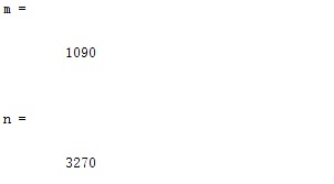
or:
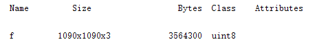
whos f
Get specific matrix information:
Three. Display image
The syntax for displaying images and CV is somewhat different:
imshow(f)
Of course, if this image is a grayscale image, you can add a grayscale number matrix G as a filter:
imshow(f, [low high])
Among them, the value below low is gray, the value above high is white, and the value in between is medium brightness value.
Of course, you can also figurecreate a form to display multiple pictures.
Four. Save the picture
It is reasonable to say that saving pictures should not be used much, just remember:
imwrite(f, 'filename')
imwrite(f,'filename.jpg', 'quality', q)
If you have been exposed to JPG images, you should know that jpg can be compressed, and q is the compression rate of 0~100
Can also be used imfinfoto view images of various information, returns a structure can be used .to access, a structure consisting of:
           Filename: 'D:\Matlab_WS\test.jpg'
        FileModDate: '17-Mar-2018 21:50:22'
           FileSize: 302838
             Format: 'jpg'
      FormatVersion: ''
              Width: 1090
             Height: 1090
           BitDepth: 24
          ColorType: 'truecolor'
    FormatSignature: ''
    NumberOfSamples: 3
       CodingMethod: 'Huffman'
      CodingProcess: 'Sequential'
            Comment: {}
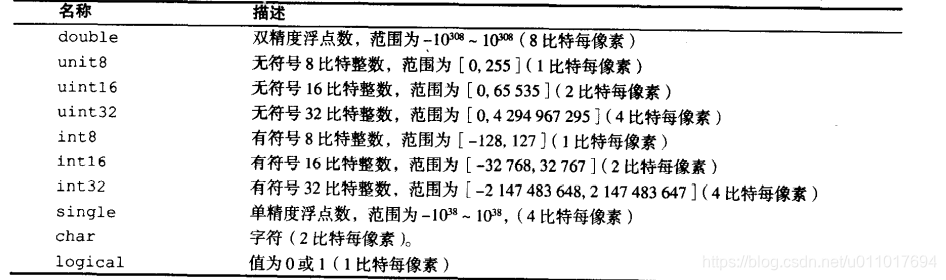
Five. Data
Not much to look at, bit-wide data types
6. Image type
6.1 Classification
The toolbox supports the following four image types:
- Brightness image
- Binary image
- Index image
- RGB image
6.2 Brightness image
In the brightness image, its brightness is represented by uint8 and uint16. In the grayscale image, the grayscale is the brightness; in other images, the brightness is the weighted value of each channel.
6.3 Binary image
As the name suggests, it is an image composed of 0 or 1. But note that in Matlab, to be considered a binary image, the data type must be a logicalclass.
Seven. Image and data conversion
7.1 Conversion of data types
For pure data type conversion, directly use the corresponding function to complete the conversion between data types:
B = ClassName(A)
The type name is from the previous table.
7.2 Conversion between image classes and types
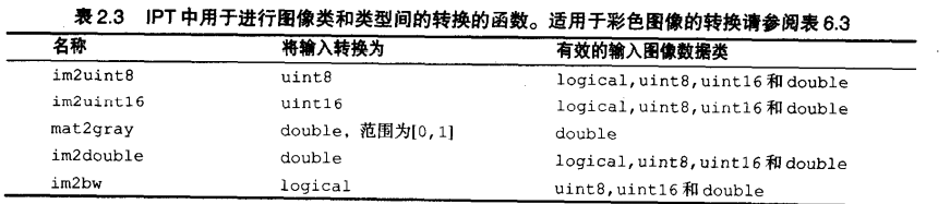
Through some function conversions, generally speaking, the maximum and minimum values of the new range are directly taken for the excess part, or the normalized value is divided by the maximum value of the new range.
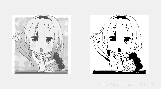
For example, here is the process of converting a brightness image to a normalized gray image and then binarizing:
f = imread('.\gray.jpg');
double_f = im2double(f);
gray_f = mat2gray(double_f);
gb_f = im2bw(gray_f, 0.6);
subplot(1,2,1);
imshow(f);
subplot(1,2,2);
imshow(gb_f);
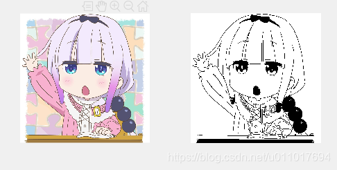
The effect of using RGB is similar, but there are some differences:
Although statements support nesting, it seems that Matlab is not as convenient as Python and C++'s OpenCV.
8. Array index
This part is similar to Python's array slicing, and the code is similar.
8.1 Vector Index
It looks like this:
v = [0 1 2 3 4 5];
v(1)
ans is displayed as ans=0
so Matlab's array starts at 1.
转置操作符 .'
v = [0 1 2 3 4 5];
v = v.'
%%
v =

     0
     1
     2
     3
     4
     5
%%
slice:
- matrix (first index: number) also supports
end
v = [0 1 2 3 4 5];
v(1:3)
v(1:end)
%%
ans =
     0     1     2
ans =
     0     1     2     3     4     5
%%
- Custom step length: matrix (first index: step length: number)
v = [0 1 2 3 4 5];
v(1:2:end)
v(end:-2:1)
%%
ans =
     0     2     4
ans =
     5     3     1
%%
- Slicing matrix: matrix([matrix])
v = [0 1 2 3 4 5];
v([1 3 5])
%%
ans =
     0     2     4
%%
8.2 Matrix Index
In the same way, slices are supported in high-dimensional matrices, and the book uses two-dimensional as the standard:
- Construction and simple subscript access
v = [0 1 2; 3 4 5; 6 7 8]
v(2,2)
%%
v =
     0     1     2
     3     4     5
     6     7     8
ans =
     4
%%
- Row and column slice
v = [0 1 2; 3 4 5; 6 7 8];
v(1:end, 2)
v(2,:)
%%
ans =
     1
     4
     7
ans =
     3     4     5
%%
You can also assign values directly without considering whether the rows and columns correspond to each other. This thing will automatically convert, and even scalars can be:
v = [0 1 2; 3 4 5; 6 7 8];
v(:, 2) = [1 2 3];
v(2,:) = 0;
v
%%
v =
     0     1     2
     0     0     0
     6     3     8
%%
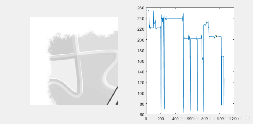
So you can extract the roiscan line of the picture or the row and column like this :
f = imread('.\gray.jpg');
roi = f(1:256, 1:256);
line = f(:,256);
subplot(1,2,1);
imshow(roi);
subplot(1,2,2);
plot(line);
8.3 Choosing the Dimension of the Array
Many operations can actually be followed by the number of dimensions they operate:
size(A, dim)
For example, in this function, dim=1 indicates the number of rows of size, and dim=2 indicates the number of columns.
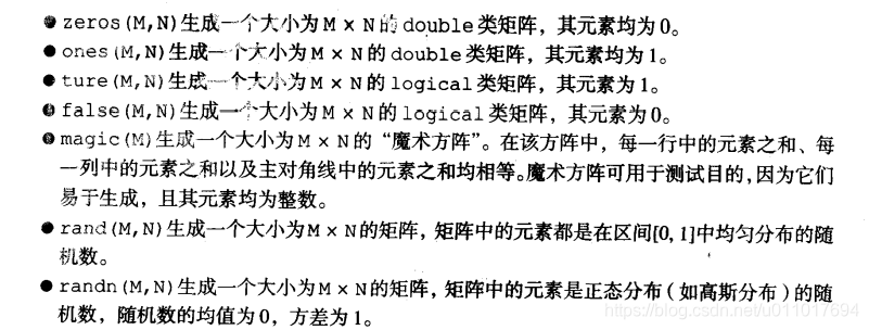
Nine. Some important standard arrays
In fact Numpy, it is similar to the code for generating some special matrices, so put the picture directly:
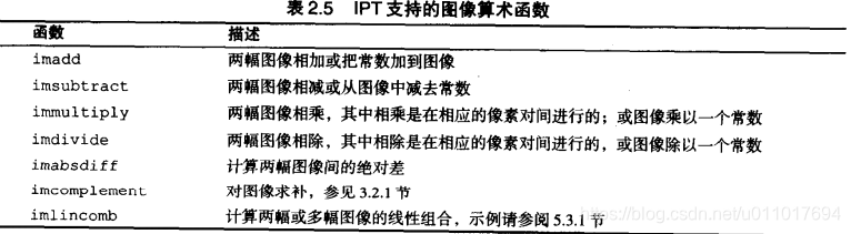
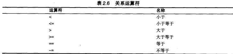
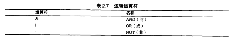
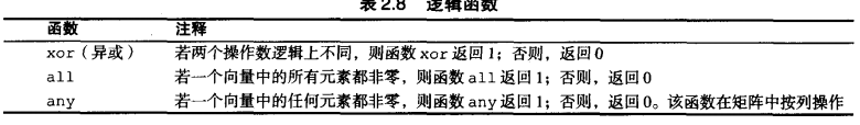
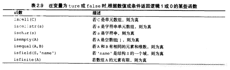
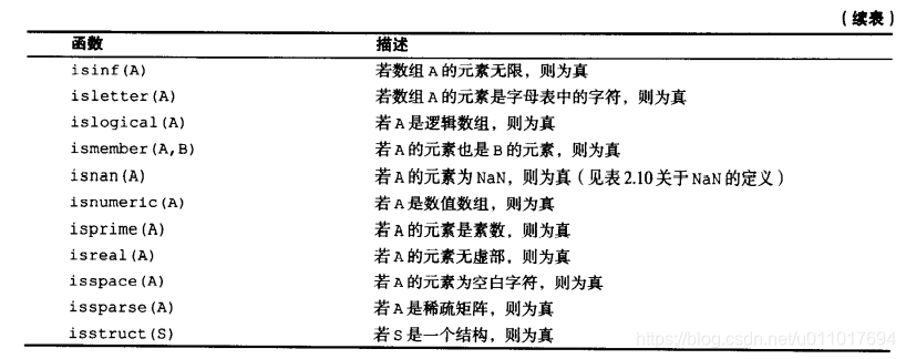
10. Operator
It also puts pictures directly, which is similar to other programming languages. So take a look and remember:

11. Flow control
11.1 if statement
if expre1
	statement1
elseif expre2
	statement2
else
	statement3
end
With this magical structure, I can feel how many programming languages this thing is a combination of. . .
11.2 for statement
for index = start:increment:end
	statements
end
E.g:
cnt = 0;
for j=0:1:10
   cnt = cnt + 1;
end
cnt
%%
cnt =
		11
%%
11.3While
while expre
	statements
end
At the same time, support continueandbreak
11.4switch
switch expre
	case condition1
		statement
	case condition2
		statement
	otherwise
		statement
end
12. Vectorization
I said earlier that it Matlabis a matrix-oriented language. After reading this part, it may be like Numpythat, adding a lot of code for optimizing the matrix, or even using GPU to calculate the matrix in parallel, so the efficiency of simply using for will be far less efficient than matrix operations. So in general, it is worth passing it to a vector or matrix. Here is an example: the time is counted by the chunks
passed ticand tocwrapped. Here is a structure of the function:
f (x, y) = A ⋅ sin (u 0 x + v 0 y) f(x,y)=A\cdot sin(u_0x+v_0y)f(x,and )=A⋅s and n ( u0x+v0y )
Suppose u0and v0 areequal to 1/(4*pi), A=1, and the picture size is 0<=x, y<=256
for loop version
u0 = 1/(4*pi);
v0 = u0;
f = [];
tic
for r = 1:256
    u0x = u0*(r-1);
    for c = 1:256
        v0y = v0*(c-1);
        f(r,c) = sin(u0x+v0y);
    end
end
t1 = toc;
imshow(f);
t1
Get the picture
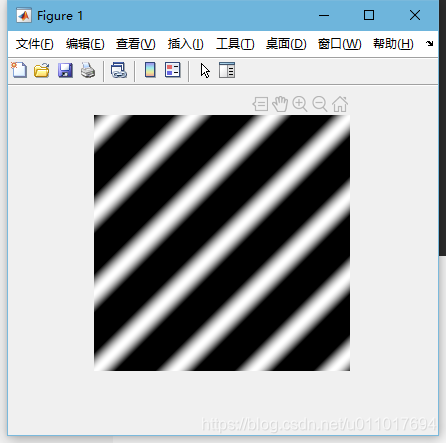
and time t1=0.0051
matrix version:
u0 = 1/(4*pi);
v0 = u0;
f = []
tic
r = 0:255;
c = 0:255;
[C, R] = meshgrid(c, r);
g = sin(u0*R + v0*C);
t1 = toc;
g = mat2gray(g);
imshow(g);
t1
The picture is the same, but the time is shortened to:t1 = 0.0011
Thirteen.IO stream
Use an output disp( )to
an input is similarPython t=input('message out')
14. Cell array and structure
This is similar to Pythonan array, any type can be added, but the value inside will not be modified.
c = {'A', 'BC', [1 2], [1 2; 3 4], 5}
c{1}
c{2}
c{3}
c{4}
c{5}
%%
c =
  1×5 cell 数组
    {'A'}    {'BC'}    {1×2 double}    {2×2 double}    {[5]}
ans =
    'A'
ans =
    'BC'
ans =
     1     2
ans =
     1     2
     3     4
ans =
     5
%%
Or we can declare the structure:
S.age = 5;
S.name = 'kanna';
S.matrix = [1 2; 3 4];
T = S;
T.matrix = T.matrix + S.matrix;
T.matrix
%%
ans =
     2     4
     6     8
%%