MATLAB reinforcement learning combat (11) use custom training loops to train reinforcement learning strategies

This example shows how to define a custom training loop for reinforcement learning strategies. You can use this workflow to train reinforcement learning strategies with your own custom training algorithm instead of using one of the built-in agents in the Reinforcement Learning Toolbox™ software.

Using this workflow, you can train strategies that use any of the following strategies and value function representations.

1. rlStochasticActorRepresentation —Random Actor Representation

2. rlDeterministicActorRepresentation —deterministic actor representation

3. rlValueRepresentation —Value function reviewer representation

4. rlQValueRepresentation — Q value function commenter representation

In this example, the REINFORCE algorithm (no baseline) is used to train a random actor strategy with discrete operating space. For more information about the REINFORCE algorithm, see Strategy Gradient Agent .

Fixed reproducibility of random generator seeds.

rng(0)

For more information about the functions available for custom training, see Custom training functions .

surroundings

For this example, the reinforcement learning strategy is trained in a discrete inverted pendulum environment. The goal in this environment is to balance the bar by applying a force (action) on the cart. Use the rlPredefinedEnv function to create an environment.

env = rlPredefinedEnv('CartPole-Discrete');

Extract observations and behavioral norms from the environment.

obsInfo = getObservationInfo(env);
actInfo = getActionInfo(env);

Get the number of observations (numObs) and the number of actions (numAct).

numObs = obsInfo.Dimension(1);
numAct = actInfo.Dimension(1);

Strategy

In this example, the reinforcement learning strategy is a discrete action stochastic strategy. It is represented by a deep neural network, which contains fullyConnectedLayer, reluLayer and softmaxLayer layers. Given the current observations, the network outputs the probability of each discrete action. softmaxLayer can ensure that the probability value range of the representation output is [0 1], and the sum of all probabilities is 1.

Create deep neural networks for actors.

actorNetwork = [featureInputLayer(numObs,'Normalization','none','Name','state')
                fullyConnectedLayer(24,'Name','fc1')
                reluLayer('Name','relu1')
                fullyConnectedLayer(24,'Name','fc2')
                reluLayer('Name','relu2')
                fullyConnectedLayer(2,'Name','output')
                softmaxLayer('Name','actionProb')];

Use the rlStochasticActorRepresentation object to create an actor representation.

actorOpts = rlRepresentationOptions('LearnRate',1e-3,'GradientThreshold',1);
actor = rlStochasticActorRepresentation(actorNetwork,...
    obsInfo,actInfo,'Observation','state',actorOpts);

For this example, the loss function of the strategy is implemented in actorLossFunction .

Use the setLoss function to set the loss function.

actor = setLoss(actor,@actorLossFunction);

Training settings

Configure training to use the following options:

1. Set the training to last up to 5000 episodes, and each episode lasts up to 250 steps.

2. To calculate the discount reward, please select a discount factor of 0.995.

3. The training is terminated when the maximum number of episodes is reached or the average reward in 100 episodes reaches a value of 220.

numEpisodes = 5000;
maxStepsPerEpisode = 250;
discountFactor = 0.995;
aveWindowSize = 100;
trainingTerminationValue = 220;

Create a vector to store the cumulative reward for each training episode.

episodeCumulativeRewardVector = [];

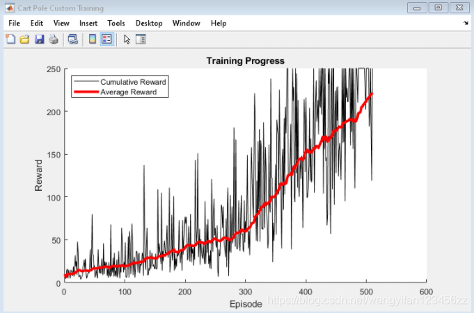
Use the hBuildFigure helper function to create a graph for training visualization.

[trainingPlot,lineReward,lineAveReward] = hBuildFigure;

Custom training loop

The algorithm of the custom training loop is as follows. For each episode:

1. Reset the environment.

2. Create a buffer for storing experience information: observations, actions, and rewards.

3. Generate experience until the final situation occurs. To do this, evaluate strategies to take measures, apply these measures to the environment, and obtain final observations and rewards. Store actions, observations and rewards in the buffer.

4. Collect training data as a batch of experience.

5. Calculate the earnings of the episode Monte Carlo, which is the future reward of the discount.

6. Calculate the gradient of the loss function according to the strategy representation parameter.

7. Use the calculated gradient to update the actor representation.

8. Update the training visualization.

9. If the strategy has been adequately trained, terminate the training.

% Enable the training visualization plot.
set(trainingPlot,'Visible','on');

% Train the policy for the maximum number of episodes or until the average
% reward indicates that the policy is sufficiently trained.
for episodeCt = 1:numEpisodes
    
    % 1. Reset the environment at the start of the episode
    obs = reset(env);
    
    episodeReward = zeros(maxStepsPerEpisode,1);
    
    % 2. Create buffers to store experiences. The dimensions for each buffer
    % must be as follows.
    %
    % For observation buffer: 
    %     numberOfObservations x numberOfObservationChannels x batchSize
    %
    % For action buffer: 
    %     numberOfActions x numberOfActionChannels x batchSize
    %
    % For reward buffer: 
    %     1 x batchSize
    %
    observationBuffer = zeros(numObs,1,maxStepsPerEpisode);
    actionBuffer = zeros(numAct,1,maxStepsPerEpisode);
    rewardBuffer = zeros(1,maxStepsPerEpisode);
    
    % 3. Generate experiences for the maximum number of steps per
    % episode or until a terminal condition is reached.
    for stepCt = 1:maxStepsPerEpisode
        
        % Compute an action using the policy based on the current 
        % observation.
        action = getAction(actor,{
    
    obs});
        
        % Apply the action to the environment and obtain the resulting
        % observation and reward.
        [nextObs,reward,isdone] = step(env,action{
    
    1});
        
        % Store the action, observation, and reward experiences in buffers.
        observationBuffer(:,:,stepCt) = obs;
        actionBuffer(:,:,stepCt) = action{
    
    1};
        rewardBuffer(:,stepCt) = reward;
        
        episodeReward(stepCt) = reward;
        obs = nextObs;
        
        % Stop if a terminal condition is reached.
        if isdone
            break;
        end
        
    end
    
    % 4. Create training data. Training is performed using batch data. The
    % batch size equal to the length of the episode.
    batchSize = min(stepCt,maxStepsPerEpisode);
    observationBatch = observationBuffer(:,:,1:batchSize);
    actionBatch = actionBuffer(:,:,1:batchSize);
    rewardBatch = rewardBuffer(:,1:batchSize);

    % Compute the discounted future reward.
    discountedReturn = zeros(1,batchSize);
    for t = 1:batchSize
        G = 0;
        for k = t:batchSize
            G = G + discountFactor ^ (k-t) * rewardBatch(k);
        end
        discountedReturn(t) = G;
    end

    % 5. Organize data to pass to the loss function.
    lossData.batchSize = batchSize;
    lossData.actInfo = actInfo;
    lossData.actionBatch = actionBatch;
    lossData.discountedReturn = discountedReturn;
    
    % 6. Compute the gradient of the loss with respect to the policy
    % parameters.
    actorGradient = gradient(actor,'loss-parameters',...
        {
    
    observationBatch},lossData);
    
    % 7. Update the actor network using the computed gradients.
    actor = optimize(actor,actorGradient);

    % 8. Update the training visualization.
    episodeCumulativeReward = sum(episodeReward);
    episodeCumulativeRewardVector = cat(2,...
        episodeCumulativeRewardVector,episodeCumulativeReward);
    movingAveReward = movmean(episodeCumulativeRewardVector,...
        aveWindowSize,2);
    addpoints(lineReward,episodeCt,episodeCumulativeReward);
    addpoints(lineAveReward,episodeCt,movingAveReward(end));
    drawnow;
    
    % 9. Terminate training if the network is sufficiently trained.
    if max(movingAveReward) > trainingTerminationValue
        break
    end
    
end

simulation

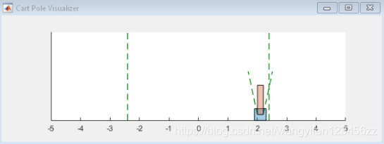
After the training, simulate the training strategy.

Please reset the environment before simulating.

obs = reset(env);

Enable environment visualization, which is updated every time the environment step function is called.

plot(env)

For each simulation step, do the following.

1. Use the getAction function to sample from the strategy to get the action.

2. Use the obtained action value to execute the environment step by step.

3. If the termination condition is reached, it terminates.

for stepCt = 1:maxStepsPerEpisode
    
    % Select action according to trained policy
    action = getAction(actor,{
    
    obs});
        
    % Step the environment
    [nextObs,reward,isdone] = step(env,action{
    
    1});
    
    % Check for terminal condition
    if isdone
        break
    end
    
    obs = nextObs;
    
end

Custom training function

To obtain the action and value function of a given observation from the strategy and value function representation of the "Reinforcement Learning Toolbox", the following functions can be used.

1. getValue — Get the estimated state value or state action value function.

2. getAction — Get the action from the actor representation based on the current observation.

3. getMaxQValue — Get the estimated maximum state action value function in the form of a discrete Q value.

If your strategy or value function representation is a recurrent neural network, that is, a neural network with at least one layer of hidden state information, the previous function can return the current network state. You can use the following function syntax to get and set the status of the representation.

1. state = getState(rep)—Get the state of the representation rep.

2. newRep = setState(oldRep, state)—Set the state of the representation oldRep and return the result in oldRep.

3. newRep = resetState (oldRep)—Reset all state values ​​of oldRep to zero, and return the result in newRep.

You can use the getLearnableParameters and setLearnableParameters functions to get and set the learnable parameters in the representation form respectively.

In addition to these functions, you can also use the setLoss, gradient, optimize, and syncParameters functions to set parameters and calculate the gradient of the strategy and value function representation.

setLoss

The strategy is trained in a stochastic gradient ascent method, where the gradient of the loss function is used to update the network. For custom training, you can use the setLoss function to set the loss function. To do this, use the following syntax.

newRep = setLoss(oldRep,lossFcn)

Here:

1. oldRep is a strategy or value function representation object.

2. lossFcn is the name of the custom loss function or the handle of the custom loss function.

3. newRep is equivalent to oldRep, except that the loss function is added to the representation.

gradient

The gradient function calculation represents the gradient of the loss function. You can calculate several different gradients. For example, to calculate the gradient of the output of a representation relative to its input, use the following syntax.

grad = gradient(rep,“output-input”,inputData)

Here:

1. rep is a strategy or value function representing an object.

2. inputData contains the value of the input channel in the form of representation.

3. grad contains the calculated gradient.

For more information, type

help rl.representation.rlAbstractRepresentation.gradient.

optimize

The optimization function updates the learnable parameters represented based on the calculated gradient. To update the gradient parameters, use the following syntax.

newRep = optimize(oldRep,grad)

Here, oldRep is the strategy or value function representation object, and grad contains the gradient calculated using the gradient function. newRep has the same structure as oldRep, but its parameters have been updated.

syncParameters

The syncParameters function is updated according to the learnable parameters represented by another form of strategy or value function. Like the DDPG agent, this feature is useful for updating the target actor or commenter's expression. To synchronize parameter values ​​between two representations, use the following syntax.

newTargetRep = syncParameters(oldTargetRep,sourceRep,smoothFactor)

Here:

1. oldTargetRep is a parameter ${\theta }_{old}$The strategy or value function represents the object.
2. sourceRep is a strategy or value function representation object, which has the same structure as oldTargetRep, but the parameter is ${\theta }_{source}$。
3. smoothFactor is the updated smoothing factor (τ).
4. newTargetRep has the same structure as oldRep, but its parameters are ${\theta }_{new}=\tau {\theta }_{source}+(1-\tau ){\theta }_{old}$。

Loss function

The loss function in the REINFORCE algorithm is the product of the discount reward and the logarithm of the strategy, and the product is summed across all time steps. The size of the discount reward calculated in the custom training loop must be adjusted to make it compatible with the multiplier strategy.

function loss = actorLossFunction(policy, lossData)

    % Create the action indication matrix.
    batchSize = lossData.batchSize;
    Z = repmat(lossData.actInfo.Elements',1,batchSize);
    actionIndicationMatrix = lossData.actionBatch(:,:) == Z;
    
    % Resize the discounted return to the size of policy.
    G = actionIndicationMatrix .* lossData.discountedReturn;
    G = reshape(G,size(policy));
    
    % Round any policy values less than eps to eps.
    policy(policy < eps) = eps;
    
    % Compute the loss.
    loss = -sum(G .* log(policy),'all');
    
end

Helper function

The following helper function creates a graph for training visualization.

function [trainingPlot, lineReward, lineAveReward] = hBuildFigure()
    plotRatio = 16/9;
    trainingPlot = figure(...
                'Visible','off',...
                'HandleVisibility','off', ...
                'NumberTitle','off',...
                'Name','Cart Pole Custom Training');
    trainingPlot.Position(3) = plotRatio * trainingPlot.Position(4);
    
    ax = gca(trainingPlot);
    
    lineReward = animatedline(ax);
    lineAveReward = animatedline(ax,'Color','r','LineWidth',3);
    xlabel(ax,'Episode');
    ylabel(ax,'Reward');
    legend(ax,'Cumulative Reward','Average Reward','Location','northwest')
    title(ax,'Training Progress');
end