Article Directory
0 Notes
Derived from [Machine Learning] [Whiteboard Derivation Series] [Collection 1~23] , I will derive on paper with the master of UP when I study. The content of the blog is a secondary written arrangement of notes. According to my own learning needs, I may The necessary content will be added.
Note: This note is mainly for the convenience of future review and study, and it is indeed that I personally type one word and one formula by myself. If I encounter a complex formula, because I have not learned LaTeX, I will upload a handwritten picture instead (the phone camera may not take the picture Clear, but I will try my best to make the content completely visible), so I will mark the blog as [original], if you think it’s not appropriate, you can send me a private message, I will judge whether to set the blog to be visible only to you or something else based on your reply. Thank you!
This blog is a note for (Series 1), and the corresponding videos are: [(Series 1) Introduction-Introduction to Information], [(Series 1) Introduction-Frequent School vs. Bayesian School].
The text starts below.
1 Data and parameters
Let the data set be X, there are N sample instances in X, and each sample has p dimensions. Symbolically expressed as X = (x 1 ,x 2 ,...,x N ) T , x i ∈ R p , i=1...N. Then X is an N*P order matrix.
When the parameter is θ, X obeys the distribution P(X|θ), denoted as X~P(X|θ). The following will introduce the different views of the frequency school and the Bayesian school on θ.
2 Frequency group: θ is an unknown constant
Frequentists believe that θ is an unknown constant and data X is a random variable; Frequentists’ approach is to estimate θ through data X.
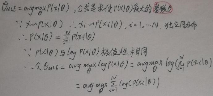
Use Maximum Likelihood Estimate (MLE) to find θ:
3 Bayesian: θ is a random variable
Bayesian believes that θ is a random variable , and that θ obeys a random distribution P(θ), that is, θ~P(θ), and P(θ) is called a priori.
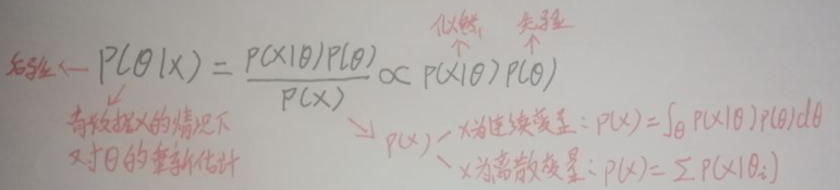
The following is Bayesian estimation:
4 Maximum posterior probability (MAP) estimation
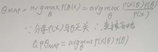
The idea of MAP (maximum posterior probability) estimation is the same as MLE (maximum likelihood estimation). It is believed that θ obeys a certain random distribution. What MAP estimation does is to find a θ to maximize the posterior probability P(X|θ):
5 Bayesian prediction
First, give a formula, which will be used later in this section: P(X=a,Y=b|Z=c)=P(X=a|Y=b,Z=c)P(Y=b|Z=c ).
The data set is X = (x 1 ,x 2 ,…,x N ) T , x i ∈ R p , i=1…N. Let x'be the new data, and build the relationship between X and x'through the bridge——θ: In the
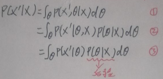
above formula, the formula mentioned at the beginning of this section is used from ① to ②; from ② to ③ x'and X Is independent, so you can directly omit X to get P(x'|θ).
When Bayesian prediction calculates P(x'|X), the posterior probability P(θ|X) must be obtained first, and Bayesian estimation is to calculate P(θ|X), which is the meaning of Bayesian estimation .
6 Summary
(1) The model obtained by Bayesian school is called a probabilistic graph model, and its essence is to integrate;
(2) The model obtained by the frequency group is called statistical machine learning, and its essence is an optimization problem (model-loss function-algorithm).
END