1 Introduction
It is relatively simple to implement any machine learning algorithm in Python using the Scikit-Learn module, and you do not need to know all the details. Here is an overview of how to perform random forest regression on the algorithm, and details on the parameters. Hope it will be helpful to your work.
Here, I will introduce how to build and use Random Forest regression in Python, instead of just showing the code, I will try to understand how the model works.
1.1 Overview of Random Forest
Random forest is a supervised machine learning algorithm based on ensemble learning. Ensemble learning is a type of learning in which different types of algorithms or the same algorithm can be added multiple times to form a more powerful predictive model. Random forest combines multiple algorithms of the same type, that is, multiple decision-making trees, hence the name "random forest".
1.2 Understanding the decision tree
Decision tree is the building block of random forest, and it is an intuitive model in itself. We can think of a decision tree as a flowchart asking questions about our data. This is an interpretable model because it determines what we do in real life: before finally reaching a decision, we will ask a series of questions about the data.
Random forest is an overall model composed of many decision trees. The prediction is made by averaging the predictions of each decision tree. Just as a forest is a collection of trees, a random forest model is also a collection of decision tree models. This makes Random Forest a powerful modeling technique, which is much more powerful than a single decision tree.
Each tree in the random forest is training on a subset of the data. The basic idea behind it is to combine multiple decision trees when determining the final output, instead of relying on individual decision trees. Each decision tree has a high variance, but when we combine all decision trees in parallel, because each decision tree is perfectly trained for specific sample data, the result variance is very low, so the output does not depend on More than one decision tree but multiple decision trees. For regression problems, the final output is the average of all decision tree outputs.
1.3 Overview of the working process of random forest
- N sample subsets are randomly selected from the data set.
- Construct a decision tree based on the N sample subsets.
- Select the number of trees required in the algorithm, and then repeat steps 1 and 2.
For regression problems, each tree in the forest will predict the Y value (output). The final value is calculated by taking the average of the predicted values of all decision trees in the forest.
1.4 Bootstrapping&Bagging
Bootstrapping
Bootstrapping algorithm refers to the use of limited sample data through multiple repeated sampling. Such as: sampling with replacement in the original sample, sampling n times. Each time a new sample is drawn, and the operation is repeated to form many new samples.
Random forest is to train a decision tree on each random sample. Although each tree may be very different from a specific set of training data, overall, the variance of the entire forest is very small.
Bagging
Random forest trains each decision tree on different randomly selected sample subsets, and then averages the predictions to make overall predictions. This process is called Bagging.
2 Advantages and disadvantages of random forest
2.1 Advantages of random forest regression
In the field of machine learning, the random forest regression algorithm is more suitable for regression problems than other common and popular algorithms.
- There is a non-linear or complex relationship between features and labels.
- It is not sensitive to noise in the training set, and is more conducive to obtaining a robust model. The random forest algorithm is more robust than a single decision tree because it uses a set of unrelated decision trees.
- Avoid overfitting models.
2.2 Disadvantages of random forest
- The main disadvantage of random forest is its complexity. Since a large number of decision trees need to be connected together, they require more computing resources.
- Due to their complexity, they require more time for training than other similar algorithms.
2.3 Overfitting problem of random forest
Underfitting, fit and overfitting are shown in the figure below. When there is an overfitting situation, the performance of the training data model is good, and the performance of the test data model is definitely poor. Machine learning is more prone to overfitting. The over-fitting problem of random forest is divided into two schools, which will produce over-fitting and not over-fitting.

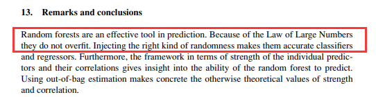
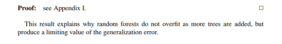
Will not overfit:
In Leo Breiman (the creator of the random forest algorithm) paper "Random Forests" statement:
Will overfit:
problem description, part of the data (90% of the data) as a training sample, a part (10% ) As a test sample, it is found that the R2 of the training sample is always 0.85, while the R2 of the test sample is only 0.5 a few, and the high is only 0.6 a few.
For this problem, it is also very likely that the relationship between the independent variable and the dependent variable itself is very low, resulting in an over-fitting artifact.
3 Practice using random forest regression
In this section, we will study how to use Scikit-Learn to apply random forests to solve regression problems.
3.1 Problem description
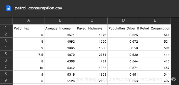
Based on gasoline taxes (in US cents), per capita income (in U.S. dollars), highways (in miles), and proportion of population to predict gasoline consumption (in millions of gallons) in the 48 states of the United States.
In order to solve this regression problem, the random forest algorithm in Scikit-Learn is used.
3.2 Sample data
The example data set is available at the following location (KeXueShangWang is required to open it):
https://drive.google.com/file/d/1mVmGNx6cbfvRHC_DvF12ZL3wGLSHD9f_/view
3.3 Code
Related explanations are commented in the code
import pandas as pd
import numpy as np

# 导入数据,路径中要么用\\或/或者在路径前加r
dataset = pd.read_csv(r'D:\Documents\test_py\petrol_consumption.csv')

# 输出数据预览
print(dataset.head())

# 准备训练数据
# 自变量:汽油税、人均收入、高速公路、人口所占比例
# 因变量:汽油消耗量
X = dataset.iloc[:, 0:4].values
y = dataset.iloc[:, 4].values

# 将数据分为训练集和测试集
from sklearn.model_selection import train_test_split

X_train, X_test, y_train, y_test = train_test_split(X,
                                                    y,
                                                    test_size=0.2,
                                                    random_state=0)

# 特征缩放,通常没必要
# 因为数据单位,自变量数值范围差距巨大,不缩放也没问题
from sklearn.preprocessing import StandardScaler

sc = StandardScaler()
X_train = sc.fit_transform(X_train)
X_test = sc.transform(X_test)

# 训练随机森林解决回归问题
from sklearn.ensemble import RandomForestRegressor

regressor = RandomForestRegressor(n_estimators=200, random_state=0)
regressor.fit(X_train, y_train)
y_pred = regressor.predict(X_test)

# 评估回归性能
from sklearn import metrics

print('Mean Absolute Error:', metrics.mean_absolute_error(y_test, y_pred))
print('Mean Squared Error:', metrics.mean_squared_error(y_test, y_pred))
print('Root Mean Squared Error:',
      np.sqrt(metrics.mean_squared_error(y_test, y_pred)))
Output result
  Petrol_tax  Average_income  Paved_Highways  Population_Driver_licence(%)  Petrol_Consumption
0         9.0            3571            1976                         0.525                 541
1         9.0            4092            1250                         0.572                 524
2         9.0            3865            1586                         0.580                 561
3         7.5            4870            2351                         0.529                 414
4         8.0            4399             431                         0.544                 410
Mean Absolute Error: 48.33899999999999
Mean Squared Error: 3494.2330150000003
Root Mean Squared Error: 59.112037818028234
4 Detailed explanation of Sklearn random forest regression parameters
To understand the sklearn.ensemble.RandomForestRegressormeaning of each parameter, we need to start from the function definition, specific description will have to see the official website description:
sklearn.ensemble.RandomForestRegressor(
n_estimators=100, *, 				# 树的棵树,默认是100
criterion='mse', 					# 默认“ mse”,衡量质量的功能,可选择“mae”。
max_depth=None, 					# 树的最大深度。
min_samples_split=2, 				# 拆分内部节点所需的最少样本数:
min_samples_leaf=1, 				# 在叶节点处需要的最小样本数。
min_weight_fraction_leaf=0.0, 		# 在所有叶节点处的权重总和中的最小加权分数。
max_features='auto', 				# 寻找最佳分割时要考虑的特征数量。
max_leaf_nodes=None, 				# 以最佳优先方式生长具有max_leaf_nodes的树。
min_impurity_decrease=0.0, 			# 如果节点分裂会导致杂质的减少大于或等于该值,则该节点将被分裂。
min_impurity_split=None, 			# 提前停止树木生长的阈值。
bootstrap=True, 					# 建立树木时是否使用bootstrap抽样。 如果为False,则将整个数据集用于构建每棵决策树。
oob_score=False, 					# 是否使用out-of-bag样本估算未过滤的数据的R2。
n_jobs=None, 						# 并行运行的Job数目。
random_state=None, 					# 控制构建树时样本的随机抽样
verbose=0, 							# 在拟合和预测时控制详细程度。
warm_start=False, 					# 设置为True时,重复使用上一个解决方案,否则,只需拟合一个全新的森林。
ccp_alpha=0.0,
max_samples=None)					# 如果bootstrap为True,则从X抽取以训练每个决策树。
5 Visualization of Random Forest
5.1 Code
import sklearn.datasets as datasets
import pandas as pd
from sklearn.model_selection import train_test_split
from sklearn.preprocessing import StandardScaler
from sklearn.pipeline import Pipeline
from sklearn.ensemble import RandomForestRegressor
from sklearn.decomposition import PCA

# 导入数据,路径中要么用\\或/或者在路径前加r
dataset = pd.read_csv(r'D:\Documents\test_py\petrol_consumption.csv')

# 输出数据预览
print(dataset.head())

# 准备训练数据
# 自变量:汽油税、人均收入、高速公路、人口所占比例
# 因变量:汽油消耗量
X = dataset.iloc[:, 0:4].values
y = dataset.iloc[:, 4].values

# 将数据分为训练集和测试集
X_train, X_test, y_train, y_test = train_test_split(X,
                                                    y,
                                                    test_size=0.2,
                                                    random_state=0)
regr = RandomForestRegressor()
# regr = RandomForestRegressor(random_state=100,
#                              bootstrap=True,
#                              max_depth=2,
#                              max_features=2,
#                              min_samples_leaf=3,
#                              min_samples_split=5,
#                              n_estimators=3)
pipe = Pipeline([('scaler', StandardScaler()), ('reduce_dim', PCA()),
                 ('regressor', regr)])
pipe.fit(X_train, y_train)
ypipe = pipe.predict(X_test)

from six import StringIO
from IPython.display import Image
from sklearn.tree import export_graphviz
import pydotplus
import os

# 执行一次
# os.environ['PATH'] = os.environ['PATH']+';'+r"D:\CLibrary\Graphviz2.44.1\bin\graphviz"
dot_data = StringIO()
export_graphviz(pipe.named_steps['regressor'].estimators_[0],
                out_file=dot_data)
graph = pydotplus.graph_from_dot_data(dot_data.getvalue())
graph.write_png('tree.png')
Image(graph.create_png())
5.2 GraphViz's executables not found error report solution
Reference blog post
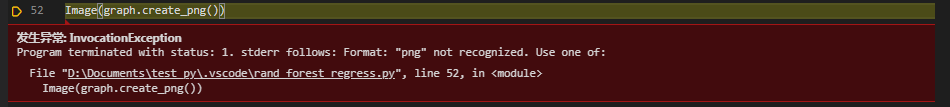
5.3 InvocationException: GraphViz's executables not found solution
Reference blog post
5.4 Visualization of Random Forest
X[0], X[1], X[2], X[3], X[4]...are the corresponding independent variables. From the structure, we can see that mse is gradually decreasing. There are a total of 12 layers of trees here, which may be much larger than the example here in actual work.

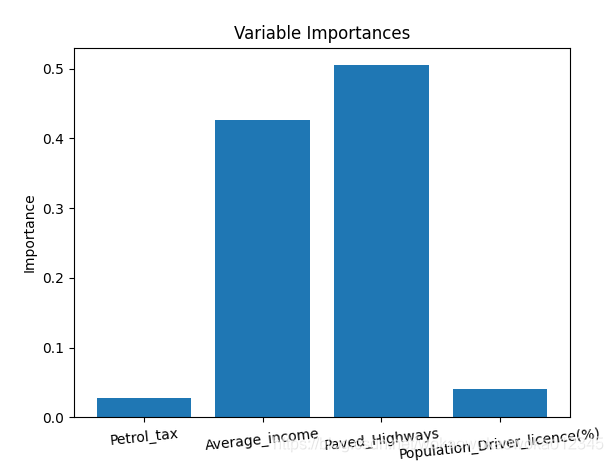
5.5 Importance of variables
Through variable importance evaluation, you can delete those unimportant variables, and the performance will not be affected. In addition, if we use different machine learning methods (such as support vector machines), we can use random forest feature importance as a feature selection method.
In order to quantify the contribution of all variables in the entire random forest to the model, we can look at the relative importance of the variables. The importance returned in Skicit-learn indicates that including specific variables can improve predictions. The actual calculation of importance is beyond the scope of this article, and only the importance value of the model output is used here.
# Get numerical feature importances
importances = list(regr.feature_importances_)
# List of tuples with variable and importance
print(importances)

# Saving feature names for later use
feature_list = list(dataset.columns)[0:4]

feature_importances = [(feature, round(importance, 2)) for feature, importance in zip(feature_list, importances)]
# Sort the feature importances by most important first
feature_importances = sorted(feature_importances, key = lambda x: x[1], reverse = True)
# Print out the feature and importances
# [print('Variable: {:20} Importance: {}'.format(*pair)) for pair in feature_importances];

# Import matplotlib for plotting and use magic command for Jupyter Notebooks

import matplotlib.pyplot as plt
# Set the style
# plt.style.use('fivethirtyeight')
# list of x locations for plotting
x_values = list(range(len(importances)))
print(x_values)
# Make a bar chart
plt.bar(x_values, importances, orientation = 'vertical')
# Tick labels for x axis
plt.xticks(x_values, feature_list,rotation=6)
# Axis labels and title
plt.ylabel('Importance'); plt.xlabel('Variable'); plt.title('Variable Importances');
plt.show()
Refer to
https://stackabuse.com/random-forest-algorithm-with-python-and-scikit-learn/
https://scikit-learn.org/stable/modules/generated/sklearn.ensemble.RandomForestRegressor.html
https: //towardsdatascience.com/random-forest-in-python-24d0893d51c0
add link description