DIP digital image processing review-feature extraction and detection chapter

Preface

This note is mainly based on the DIP theory ➕openCV implementation. To study this note, you must first make sure to read the DIP theory thoroughly, describe the relevant knowledge in your own words, and master the relevant operators in openCV

Here is mainly based on VS2017/2019 to realize the operation of openCV3.4.10 version

Image processing is divided into traditional image processing and deep learning-based image processing.When a certain chapter or section involves deep learning, I will add (deep learning) after the title to distinguish it.

Chapter One Feature Extraction

In feature extraction, traditional image processing is designed to extract fixed features by itself. In deep learning, CNN networks are mainly used to widely extract image features. In this chapter, the classics of traditional image processing are mainly introduced. Feature description and extraction methods, such as Haar, LBP, SIFT, HOG, and DPM features, where DPM features are the ceiling of traditional DIP in the field of feature extraction.

The shallow features of the image are mainly color, texture and shape

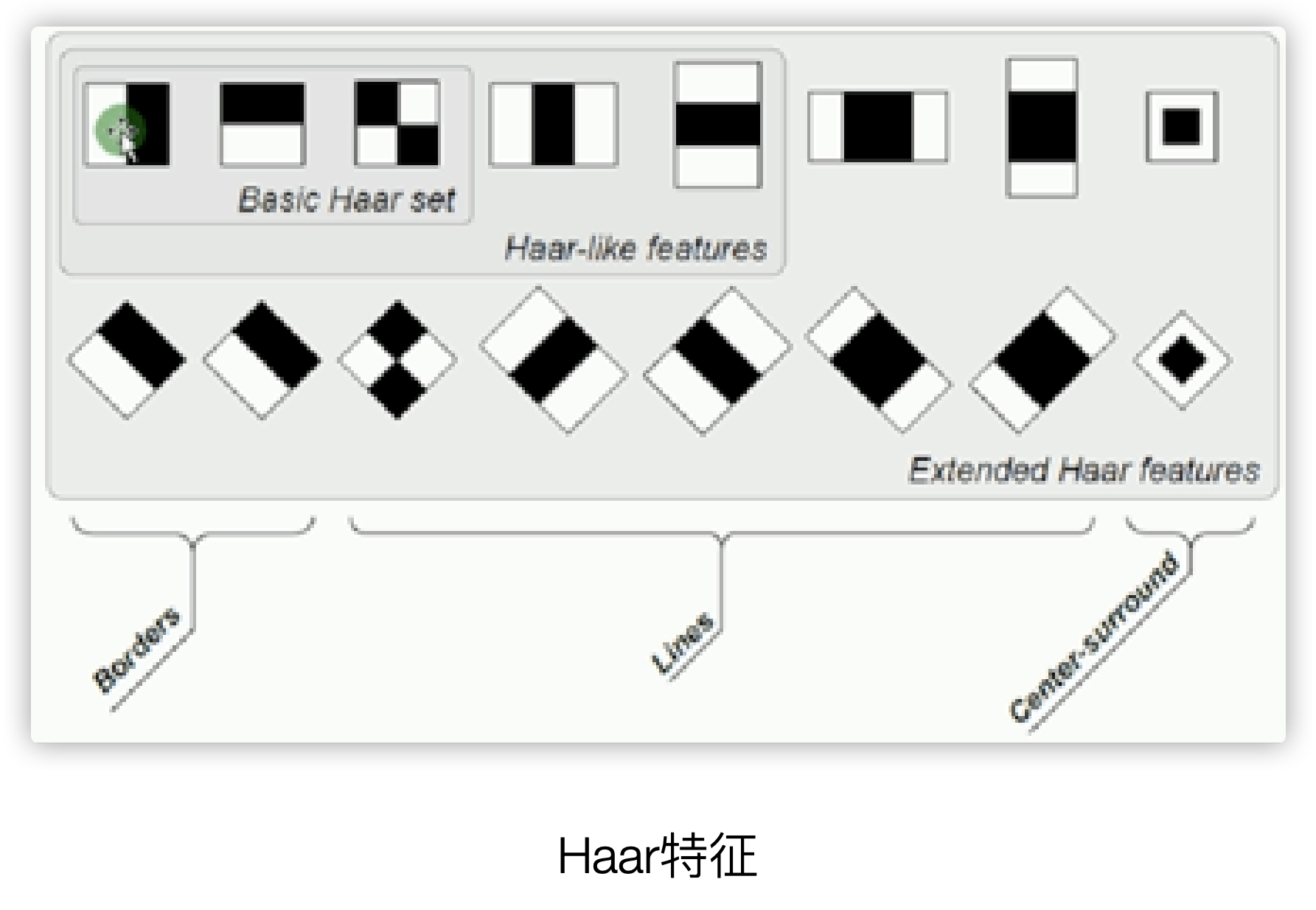
The first section Haar features ( black and white blocks )

The Haar feature is based on black and white pixel areas. Each black or white area is a pixel block containing multiple pixels. The difference between the pixel blocks determines which types of edges exist between which blocks, such as the following figure The first is the vertical edge of the description, and the second is the horizontal edge.

A rectangular Haar feature defines the difference between the sum of pixels in several areas in the rectangle, which can be any size and any position. This difference indicates some characteristics of a specific area of ​​the image

Haar features are often used in face recognition scenarios

Section 2 LBP features ( local binary mode )

LBP is the abbreviation of Local Binary Pattern, the LBP feature describes the local features of the image, and the LBP feature is characterized by rotation invariance and grayscale invariance

Commonly used in face recognition and target detection

The rotation invariance and gray invariance of LBP can often be robust to lighting, rotation, etc.

2.1 Original LBP features

In a picture or a region of interest, its LBP feature has the following description steps:

1. In a grayscale image, in the 3x3 pixel neighborhood, the center pixel is used as the threshold T, and the 8 values ​​of the 8 neighborhood pixels of the center point are compared with T respectively. If it is greater than T, it is set to 1, and if it is less than 0
2. Arrange the 8 comparison results of the first step in a row to form an 8-bit binary sequence and convert it into a decimal value
3. The decimal result is the LBP characteristic value of the center pixel

Obviously, one pixel can generate 2^8=256 LBP feature values

Because the original LBP uses fixed neighborhood pixels as the comparison object, it often loses robustness when facing size transformation, let alone rotation invariance.

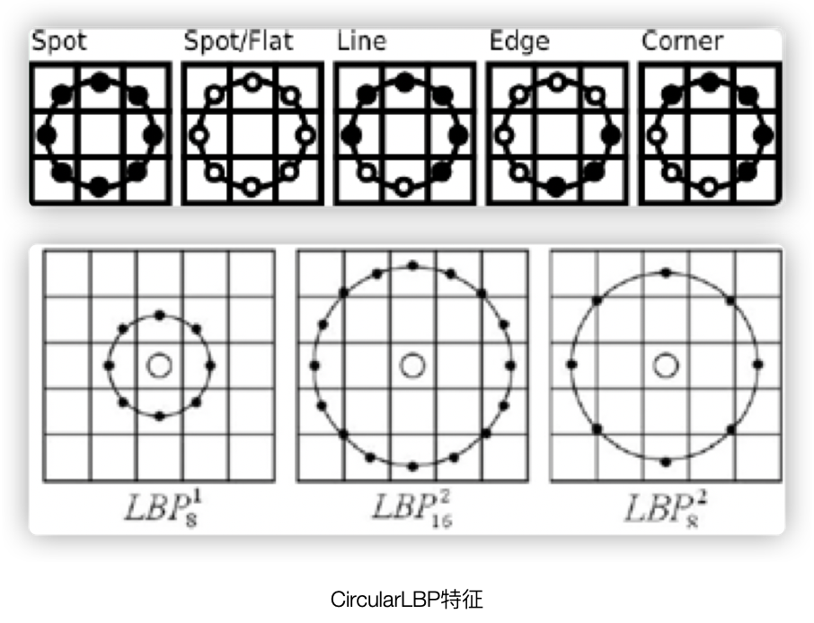
2.2 CircularLBP features

The original LBP has no rotation invariance and scale invariance, so it is improved.

In the features of CircularLBP, the basic idea of ​​LBP is retained, with the following description steps:

1. In a grayscale picture, take a certain pixel as the center point and draw a circle with R as the radius. The pixels covered by the circumference of the circle are the pixels to be compared with the center point.
2. If the pixels covered by the circumference are not in the image, the difference algorithm must be used, which is generally a bilinear difference.
3. For the neighboring pixels covered by the circle described by CircularLBP, rotate the angle according to a certain step length to obtain a series of sequences (the white point in the figure below is 1 and the black point is 0), which is converted into the LBP value, then each pixel will have Multiple LBP values
4. Take the smallest value among the above LBP values ​​as the CircularLBP feature value of the center pixel

 

 

Section 3 SIFT features ( invariant scale rotation )

SIFT is an abbreviation for scale rotation invariance, which is mainly used for the description and extraction of local features. The SIFT descriptor has strong robustness when the features are changed by rotation, scale change, scaling, and brightness in the picture.

2.3.1 SIFT feature extraction method

First, the flow chart of SIFT feature extraction is directly given, and then analyzed one by one

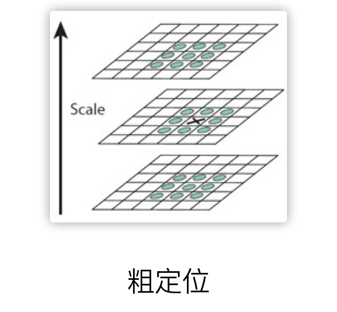
The establishment of the scale space is mainly divided into two steps.The first step is to perform the Gaussion pyramid operation on the picture. Each time the normal pyramid is downsampled, it is 1 layer, but it is called a group here. For each group of pictures, they are layered according to the fuzzy scale. , The second step is to perform pixel difference operations on the upper and lower images in each group to obtain the Gaussian difference pyramid DOG pyramid

In the flowchart, the second big step is to find the extreme point. In each octave, look for 26 neighborhood pixels in the 3x3x3 neighborhood of each pixel, and find its max or min. This extreme point is temporarily Key point

The third big step is to accurately locate the above-mentioned coarse positioning. Here, the sub-pixel level difference processing is mainly used to obtain accurate key point position information.

The fourth step is the initial assignment of the direction of the key points. This is the basis of rotation invariance. First, each key point is drawn with a radius of 3.05σ, and all the pixels covered by the circular area are calculated, and the corresponding gradient is calculated. Get the gradient direction from the size, count the 0-360° gradient direction histogram of the area, and divide 360° into 36 bins, each bin represents 10°, the direction of the histogram peak is the main direction of the key point, and the peak value is 80. The angle of% is the auxiliary direction of the key point.

The last step is the most important, that is, accurate direction calibration of the key points. At this time, accurate position information + scale information + coarse direction information has been obtained. Therefore, the direction needs to be accurately corrected. The method steps are as follows:

1. Enhance rotation invariance, take the key point as the center, and rotate the coordinate axis in the neighborhood pixel to the main direction angle of the key point to obtain new coordinates
2. In the new coordinates, take the key point as the center to obtain a 16x16 pixel window
3. In the window, 4x4 pixels are used as 1 cell, which is divided into 4x4 cells.
4. Count the gradient histogram of 16 pixels in each cell, and divide 360° into 8 bins by 45°, that is, each cell can get 8 feature information
5. This key point, in the 16x16 pixel neighborhood, a total of 16x8=128 gradient feature information is obtained, that is, each key point will generate a 128-dimensional SIFT feature vector

2.3.2 Implementation method of SIFT feature in openCV

Simple operator api is still used in openCV to achieve

cv::xfeatures2d::SIFT::create(int nfeatures = 0, 关键点总个数
				int nOctaveLayers =3, octave层数
				double contrastThreshold = 0.04, 对比度阈值 
				double edgeThreshold= 10, 边缘阈值
				double sigma=1.6)高斯模糊因子σ

The fourth section HOG features ( gradient histogram )

HOG is the abbreviation of Histograms of Oriented Gradients

The application of HOG in SVM has achieved great success in the field of pedestrian detection in traditional image processing, and it can be said to be the cornerstone of traditional pedestrian detection.

In general, in pedestrian detection, due to the obvious differences in the intrinsic characteristics of each person, a descriptor that can fully describe the characteristics of the human body is required for description, and HOG is designed based on this basic idea.

The HOG operator believes that the appearance and shape of the local target can be well described by the gradient or the direction density distribution of the edge (of course, the gradient is a gradient, and the gradient often exists at the edge)

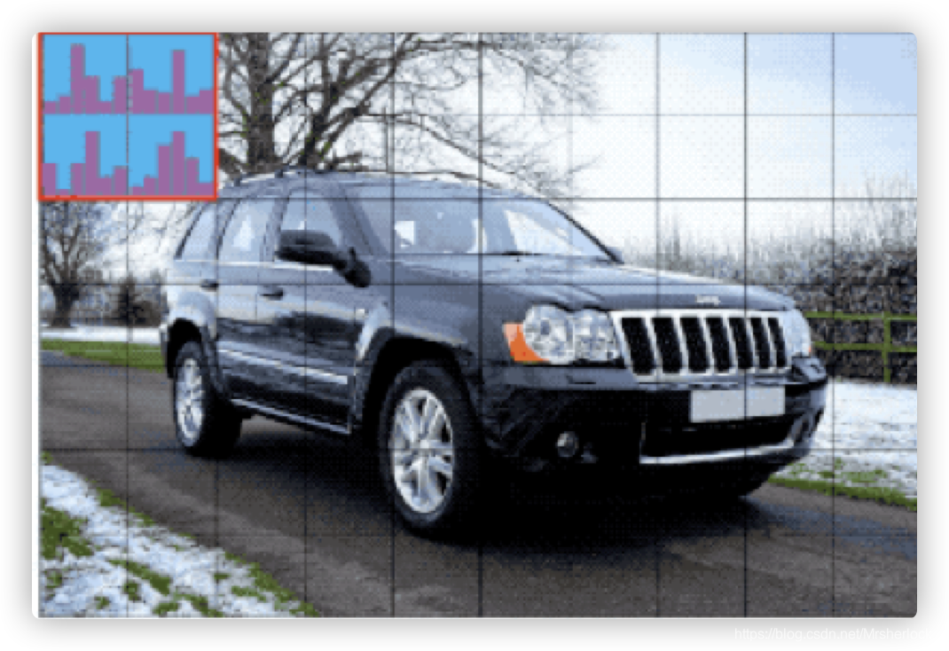
The process of HOG feature extraction is to draw the gradient distribution histogram of the image, and then use the algorithm to normalize the gradient histogram. It is this normalization algorithm that will effectively detect where the edge is. After standardization, The gradient histogram will be compressed into a feature vector, which is the HOG feature descriptor, which stores a large amount of edge information and finally serves as the input of the SVM classifier

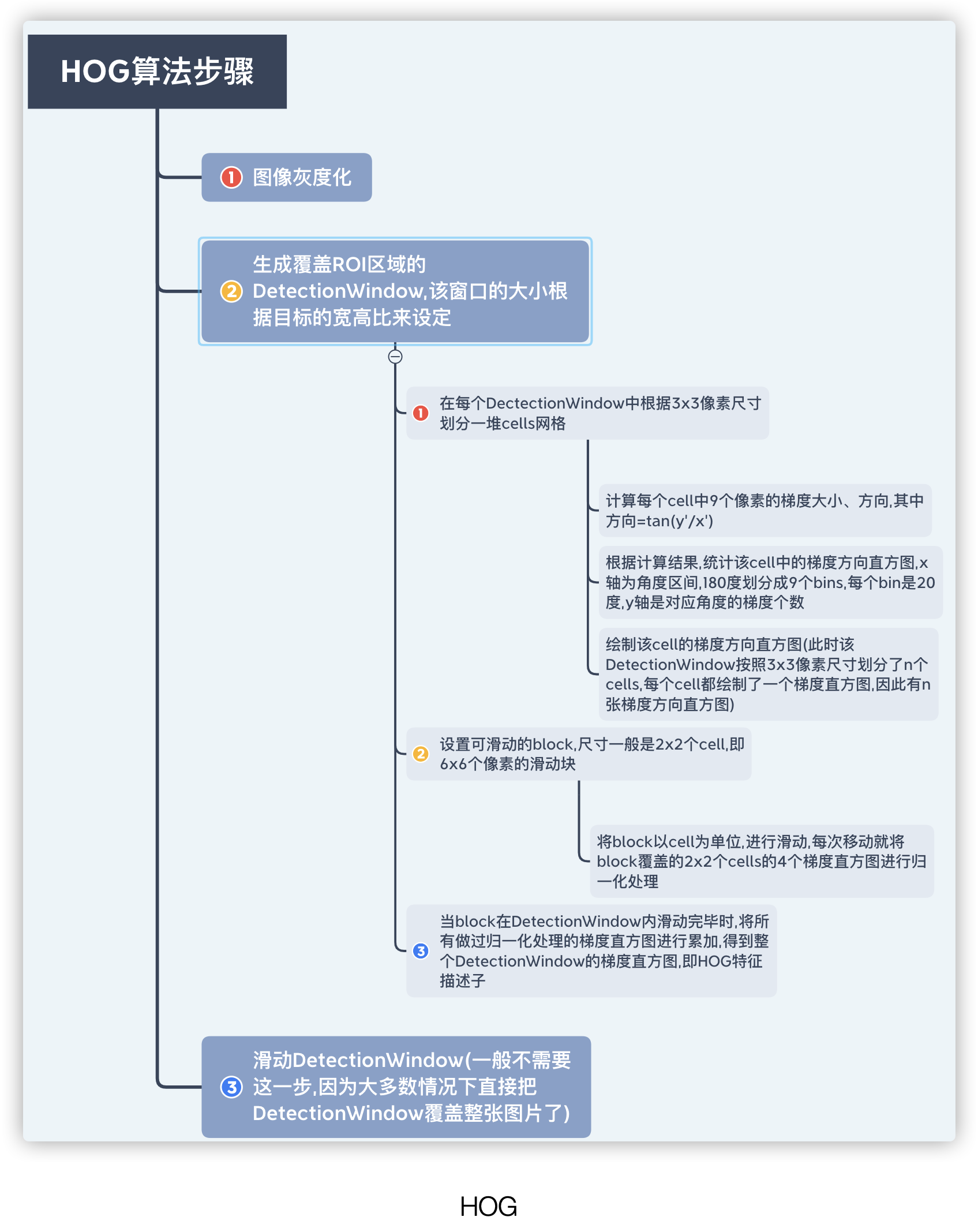
In order to better understand HOG, use the following figure to describe the processing process of the HOG descriptor

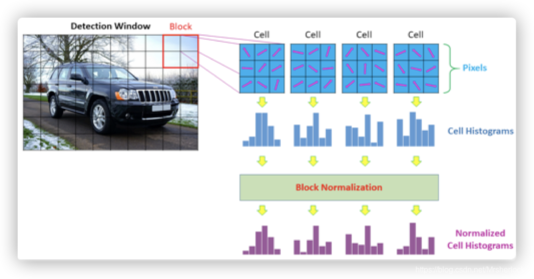
According to the above figure, the length of a HOG descriptor = the number of blocks ✖️ the number of cells covered by a block ✖️ the number of bins in the histogram of each cell.

If a picture contains multiple DetectionWindow, then the length of the HOG descriptor in a picture = the number of windows✖️The length of a HOG descriptor

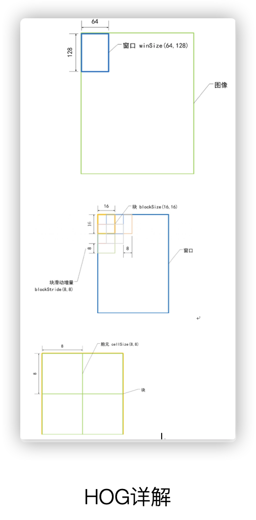
In openCV, a case about the HOG descriptor is provided, such as the following pedestrian detection case. In the following case, HOGDescriptor is the class of the HOG descriptor, hog is the class object, and the constructor of this class is the default constructor. HOGDescriptor The class has a public property of svmDetector, which is used to configure the coefficient value of the SVM classifier input to the HOG descriptor.

In the above hog class object, a 64*128, DetectionWindow, 16*16 block, 8*8 cell are constructed by default, and the HOG of each cell contains 9 bins.

For more descriptions of the HOGDescriptor class, please see: https://docs.opencv.org/3.4.10/d5/d33/structcv_1_1HOGDescriptor.html#ac0544de0ddd3d644531d2164695364d9

Case explanation:

Mat gray;
Mat dst;
resize(src, dst, Size(64,128));
cvtColor(dst, gray, COLOR_BGR2GRAY);
HOGDescriptor detector(Size(64,128), Size(16,16), Size(8,8), Size(8,8), 9);

vector<float> descriptors;
vector<Point> locations;

detector.compute(gray, descriptors, Size(0,0),Size(0,0),locations);
cout<<“result number of HOG = “<<descriptors.size()<<endl;

API introduction:

// HOG描述子
cv2.HOGDescriptor(  win_size = (64, 128),   //前5个最常用
                    block_size = (16, 16), 
                    block_stride = (8, 8), //这个是块之间的x距离和y距离
                    cell_size = (8, 8), 
                    nbins = 9, 
                    win_sigma = DEFAULT_WIN_SIGMA, 
                    threshold_L2hys = 0.2, 
                    gamma_correction = true, 
                    nlevels = DEFAULT_NLEVELS)
// 计算描述子数值类方法
HOGDescriptor::compute(image) //输入图像

virtual void cv::HOGDescriptor::compute 
(
InputArray img,
std::vector< float > &descriptors,//输出HOG描述子
Size winStride = Size(),  //窗口与窗口之间的距离
Size padding = Size(),    //窗口的步长
const std::vector< Point > &locations = std::vector< Point >()d
)const

Section 5 DPM features ( deformable component model )

DPM feature is a deformable parts model of Deformable Parts Model. DPM is the ceiling of traditional target detection algorithm. It is an extension and improvement of HOG feature detection algorithm. Since HOG often brings high-latitude feature vectors, these feature vectors are used as the input of SVM classifier. , Often produces a large amount of calculation.HOG generally uses PCA principal component analysis to reduce dimensionality, but DPM, as an improvement of the HOG algorithm, adopts a dimensionality reduction method that approximates PCA.

First of all, the premise is stipulated.DPM divides the gradient direction into signed and unsigned according to 180 degrees and 360 degrees.The sign indicates that there are positive and negative signs, and the gradient of the 0-360 angle range is regarded as directional, which is divided into 18 The bins, 0-180, are divided into 9 bins without direction. Obviously, there is no direction, and the angle of each bin is 20 degrees.

There may be deviations in the understanding of the process, but the final result is the same. Another angle of understanding is:

1. Using HOG's cell idea, every 8✖️8 pixels is a cell, the image is divided into multiple cells, the gradient size and direction of all pixels are calculated, and the gradient histogram of all pixels in each cell is counted
2. For the 4 cells in the 4 neighborhoods of each cell, that is, 4 cells on the diagonal, as shown in Figure 1234 (the green block in the figure above is the internal situation of a cell, and the yellow block is a simple stroke of the cell), and the cell and the 4 neighbors The 4 cells of the domain correspond to normalization processing, see the next step
3. The center cell and the 4 cells in the 4 neighborhoods are respectively normalized processing steps:
   • For signed gradient: Calculate the gradient direction histogram of the center cell and the i-th cell (i=1,2,3,4). In the signed gradient direction histogram, there are 18 bins, and the 4 cell histograms are accumulated 18 bins are 18 features
   • For the unsigned gradient: on the right side of the figure, the orange block in the above figure, that is, the 36 features, is regarded as a matrix, and the row summation and column summation are performed, and a total of 4+9=13 features are obtained**
   • After normalization, a total of 18+13=31 features is obtained, that is, each 8✖️8 pixel cell will generate a 31-dimensional feature vector

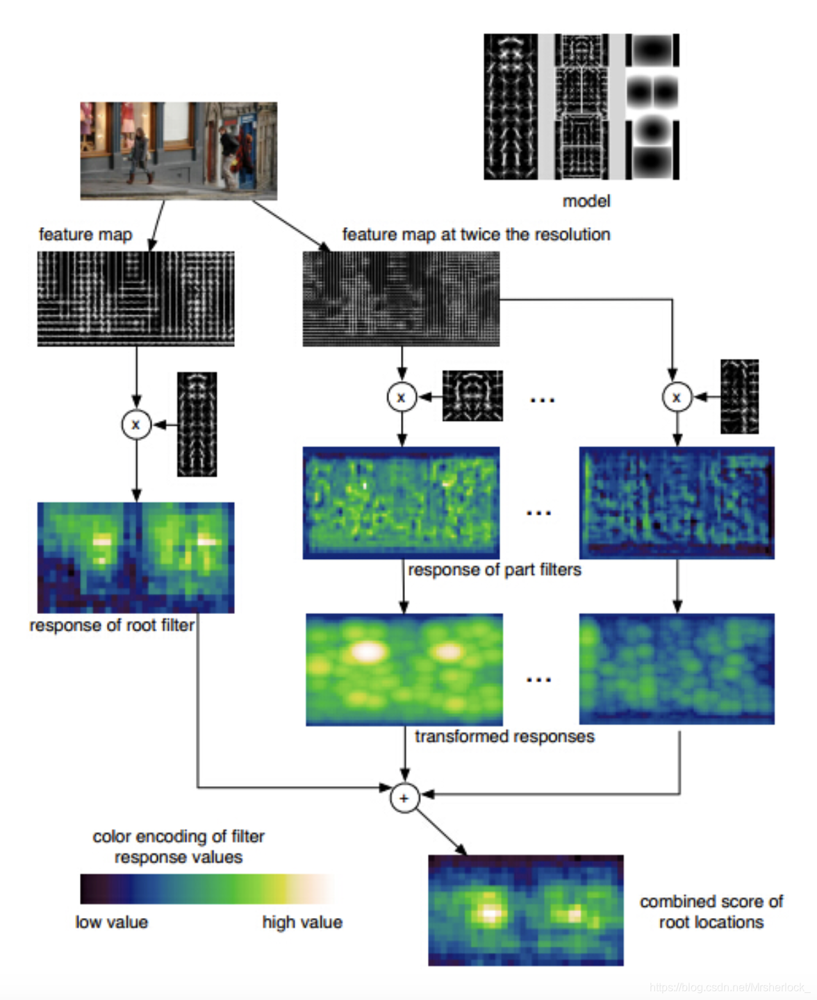
DPM detection

As the ceiling of the target detection algorithm, DPM has its own unique detection process, as shown in the following figure: