Traffic sign classification-TensorFlow implementation

Sorted out and translated from: https://github.com/waleedka/traffic-signs-tensorflow
traffic sign classification-tensorflow implementation

The test platform is win10 system, python3 operating environment, and tensorflow-gpu needs to be configured.

First introduce the necessary libraries

import os
import random
import skimage.data
import skimage.transform
import matplotlib
import matplotlib.pyplot as plt
import numpy as np
import tensorflow as tf

# Allow image embeding in notebook
%matplotlib inline

Data set analysis

Data directory structure:

/traffic/datasets/BelgiumTS/Training/
/traffic/datasets/BelgiumTS/Testing/

There are 62 sub-directories under the training set and test set, with names ranging from 00000 to 00061.
The name of the catalog represents tags from 0 to 61, and the images in each catalog represent the traffic signs belonging to that tag.
The image storage format is .ppm format, which can be read using the skimage library.

def load_data(data_dir):
    """Loads a data set and returns two lists:

    images: a list of Numpy arrays, each representing an image.
    labels: a list of numbers that represent the images labels.
    """
    # Get all subdirectories of data_dir. Each represents a label.
    directories = [d for d in os.listdir(data_dir) 
                   if os.path.isdir(os.path.join(data_dir, d))]
    # Loop through the label directories and collect the data in
    # two lists, labels and images.
    labels = []
    images = []
    for d in directories:
        label_dir = os.path.join(data_dir, d)
        file_names = [os.path.join(label_dir, f) 
                      for f in os.listdir(label_dir) if f.endswith(".ppm")]
        # For each label, load it's images and add them to the images list.
        # And add the label number (i.e. directory name) to the labels list.
        for f in file_names:
            images.append(skimage.data.imread(f))
            labels.append(int(d))
    return images, labels

# Load training and testing datasets.
ROOT_PATH = ""
train_data_dir = os.path.join(ROOT_PATH, "datasets/BelgiumTS/Training")
test_data_dir = os.path.join(ROOT_PATH, "datasets/BelgiumTS/Testing")

images, labels = load_data(train_data_dir)

Print out all the pictures and the number of labels

print("Unique Labels: {0}\nTotal Images: {1}".format(len(set(labels)),

len(images)))
Unique Labels: 62
Total Images: 4575

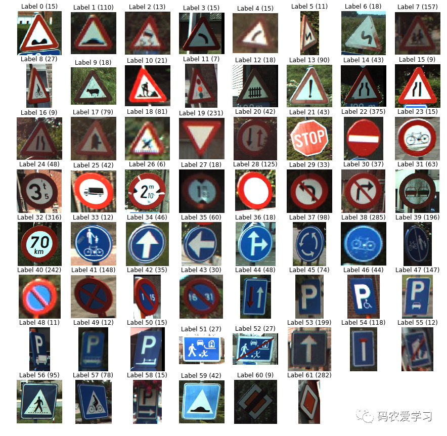
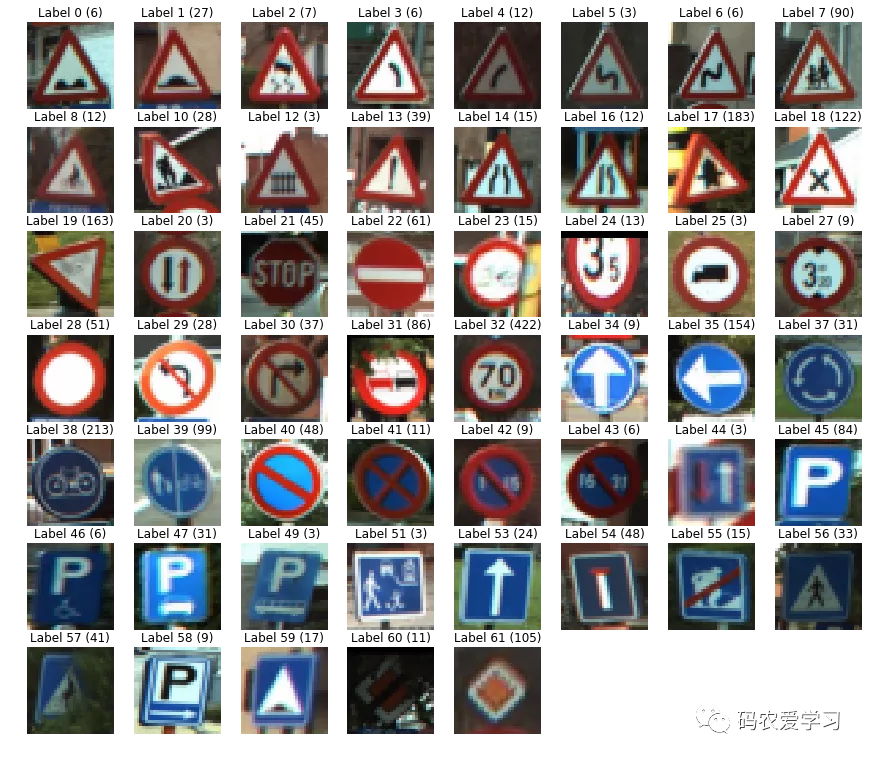
Display the first picture of each type of label

def display_images_and_labels(images, labels):
    """Display the first image of each label."""
    unique_labels = set(labels) # set：不重复出现
    plt.figure(figsize=(15, 15)) # figure size
    i = 1
    for label in unique_labels:
        # Pick the first image for each label.
        image = images[labels.index(label)] #每个label在整个labels表中的位置
        # str1.index(str2, beg=0, end=len(string)) str2在str1中的索引值
        # print(labels.index(label))
        plt.subplot(8, 8, i)  # A grid of 8 rows x 8 columns
        plt.axis('off')
        plt.title("Label {0} ({1})".format(label, labels.count(label)))# label，totalnum
        i += 1
        _ = plt.imshow(image)
    plt.show()

display_images_and_labels(images, labels)

Although the picture is square, the aspect ratio of each picture is different. The input size of the neural network is fixed, so some processing needs to be done. Take a label picture before processing, and look at a few more pictures under the label, such as label 32, as follows:

def display_label_images(images, label):
    """Display images of a specific label."""
    limit = 24  # show a max of 24 images
    plt.figure(figsize=(15, 5))
    i = 1

    start = labels.index(label)
    end = start + labels.count(label)# count:统计字符串里某个字符出现的次数
    for image in images[start:end][:limit]:
        plt.subplot(3, 8, i)  # 3 rows, 8 per row
        plt.axis('off')
        i += 1
        plt.imshow(image)
    plt.show()

display_label_images(images, 32)

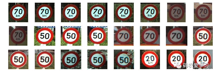
From the above pictures, we can find that although the speed limits are different, they are all grouped into the same category. This is very good, we can ignore the concept of numbers in subsequent procedures. This is why it is so important to understand your data set in advance and can save you a lot of pain and confusion in subsequent work.

So what is the size of the original picture? Let's print some first:
(Tips: print min() and max() values. This is an easy way to verify the range of your data and find errors early)

for image in images[:5]:
    print("shape: {0}, min: {1}, max: {2}".format(image.shape, image.min(),
            image.max()))

shape: (141, 142, 3), min: 0, max: 255
shape: (120, 123, 3), min: 0, max: 255
shape: (105, 107, 3), min: 0, max: 255
shape: (94, 105, 3), min: 7, max: 255
shape: (128, 139, 3), min: 0, max: 255

The size of the picture is about 128 128, then we can use this size to save the picture, so that we can save as much information as possible. However, in the early development, using a smaller size, the training model will be fast, and it can be iterated faster.
Choose the size of 32 32, it is easy to recognize the picture under the naked eye (see the picture below), and we want to ensure that the reduction ratio is a multiple of 128 * 128.

# Resize images
images32 = [skimage.transform.resize(image, (32, 32))
                for image in images]
display_images_and_labels(images32, labels)

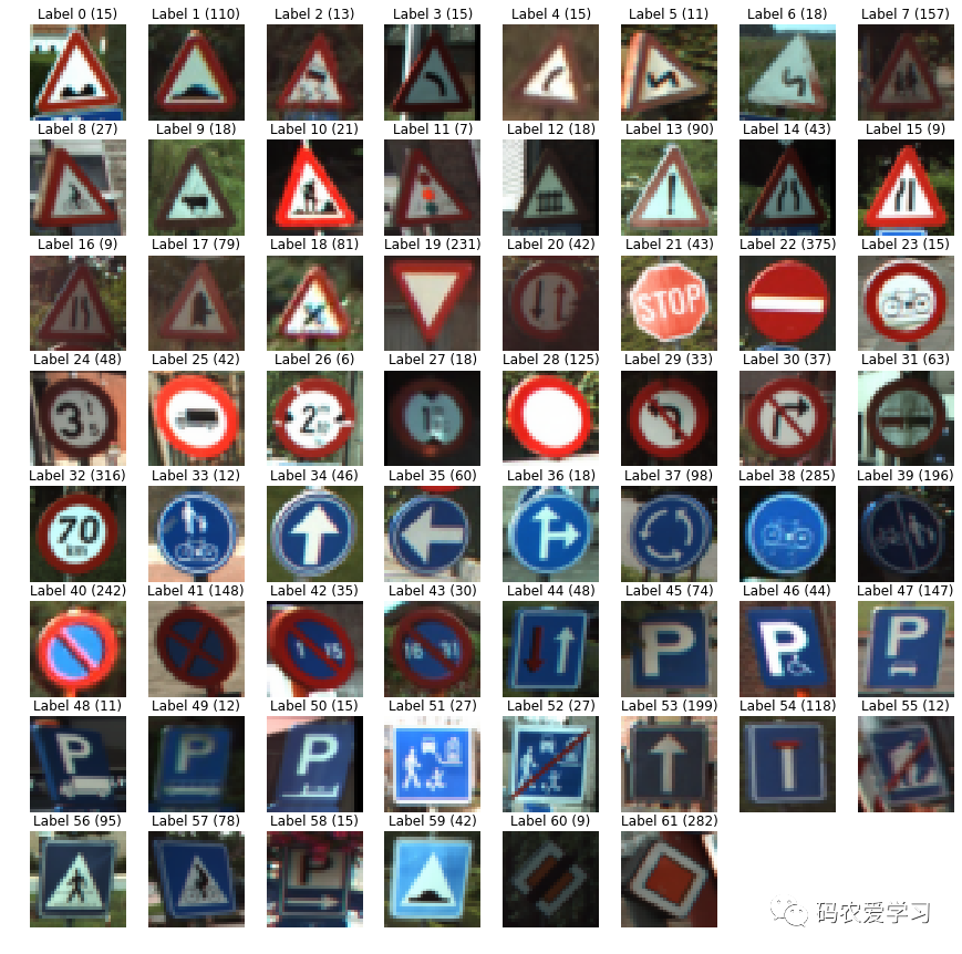
The 32x32 image is not so clear, but it is still recognizable. Note that the display above shows images larger than the actual size because the matplotlib library tries to match them to the grid size.

Let's print the size of some images to verify that we are correct.

for image in images32[:5]:
    print("shape: {0}, min: {1}, max: {2}".format(image.shape, image.min(), image.max()))

shape: (32, 32, 3), min: 0.03529411764705882, max: 0.996078431372549
shape: (32, 32, 3), min: 0.033953737745098134, max: 0.996078431372549
shape: (32, 32, 3), min: 0.03694182751225489, max: 0.996078431372549
shape: (32, 32, 3), min: 0.06460056678921595, max: 0.9191425398284313
shape: (32, 32, 3), min: 0.06035539215686279, max: 0.9028492647058823

The size is correct. But please check the minimum and maximum values! They now range from 0 to 1.0, which is different from the 0-255 range we saw above. The scaling function does this transformation for us. Normalizing the value to the range of 0-1.0 is very common, so we will keep it. But remember, if you want to convert the image back to the normal 0-255 range, multiply by 255.

labels_a = np.array(labels) # 标签
images_a = np.array(images32) # 图片
print("labels: ", labels_a.shape, "\nimages: ", images_a.shape)

labels:  (4575,) 
images:  (4575, 32, 32, 3)

Model building

First create a Graph object.

Then set up a placeholder (Placeholder) to place pictures and labels. Placeholders are the way TensorFlow receives input from the main program.
The dimension of the parameter images_ph is [None, 32, 32, 3]. These four parameters represent [batch size, height, width, channel] (usually abbreviated as NHWC). The batch size is represented by None, which means that the batch size is flexible, that is, data of any batch size can be imported into the model without modifying the code.

The output of the fully connected layer is a logarithmic vector of length 62. The output data may look like this: [0.3, 0, 0, 1.2, 2.1, 0.01, 0.4, ... ..., 0, 0]. The higher the value, the more likely the picture represents the label. The output is not a probability, they can be any value, and the result of the addition is not equal to 1. The actual value of the output neuron is not important, because it is only a relative value, relative to 62 neurons. If necessary, we can easily use the softmax function or other functions to convert into probabilities (not needed here).

In this project, you only need to know the index corresponding to the maximum value, because this index represents the classification label of the picture. The output result of the argmax function will be an integer in the range [0, 61].

The loss function uses the cross-entropy calculation method, because the cross-entropy is more suitable for classification problems, and the squared difference is suitable for regression problems.
Cross entropy is a measure of the difference between two probability vectors. Therefore, we need to convert the label and the output of the neural network into a probability vector. There is a sparse_softmax_cross_entropy_with_logits function in TensorFlow to achieve this operation. This function takes the label and the output of the neural network as input parameters, and does three things: first, convert the dimension of the label to [None, 62] (this is a 0-1 vector); second, use the softmax function to The label data and neural network output results are converted into probability values; third, the cross entropy between the two is calculated. This function will return a vector with dimension [None] (vector length is the batch size), and then we use the reduce_mean function to get a value that represents the final loss value.

The adjustment of the model parameters uses the gradient descent algorithm. The learning rate of 0.08 is more appropriate after the experiment, and the iteration is 800 times.

# Create a graph to hold the model.
graph = tf.Graph()

# Create model in the graph.
with graph.as_default():
    # Placeholders for inputs and labels.
    images_ph = tf.placeholder(tf.float32, [None, 32, 32, 3])
    labels_ph = tf.placeholder(tf.int32, [None])

    # Flatten input from: [None, height, width, channels]
    # To: [None, height * width * channels] == [None, 3072]
    images_flat = tf.contrib.layers.flatten(images_ph)

    # Fully connected layer. 【全连接层】
    # Generates logits of size [None, 62]
    logits = tf.contrib.layers.fully_connected(images_flat, 62, tf.nn.relu)

    # Convert logits to label indexes (int).
    # Shape [None], which is a 1D vector of length == batch_size.
    predicted_labels = tf.argmax(logits, 1)

    # Define the loss function. 【损失函数】
    # Cross-entropy is a good choice for classification. 交叉熵
    loss = tf.reduce_mean(tf.nn.sparse_softmax_cross_entropy_with_logits(logits=logits, labels=labels_ph))

    # Create training op.  【梯度下降算法】
    train = tf.train.GradientDescentOptimizer(learning_rate=0.08).minimize(loss)

    # And, finally, an initialization op to execute before training.
    # TODO: rename to tf.global_variables_initializer() on TF 0.12.
    init = tf.global_variables_initializer()

print("images_flat: ", images_flat)
print("logits: ", logits)
print("loss: ", loss)
print("predicted_labels: ", predicted_labels)
print(tf.nn.sparse_softmax_cross_entropy_with_logits(logits=logits, labels=labels_ph))

images_flat:  Tensor("Flatten/flatten/Reshape:0", shape=(?, 3072), dtype=float32)
logits:  Tensor("fully_connected/Relu:0", shape=(?, 62), dtype=float32)
loss:  Tensor("Mean:0", shape=(), dtype=float32)
predicted_labels:  Tensor("ArgMax:0", shape=(?,), dtype=int64)
Tensor("SparseSoftmaxCrossEntropyWithLogits_1/SparseSoftmaxCrossEntropyWithLogits:0", shape=(?,), dtype=float32)

training

# Create a session to run the graph we created.
session = tf.Session(graph=graph)

# First step is always to initialize all variables. 
# We don't care about the return value, though. It's None.
_ = session.run([init])

for i in range(801):
    _, loss_value = session.run([train, loss], 
                                feed_dict={images_ph: images_a, labels_ph: labels_a})
    if i % 20 == 0:
        print("Loss: ", loss_value)

Loss:  4.237691
Loss:  3.4573376
Loss:  3.081502
Loss:  2.89802
Loss:  2.780877
Loss:  2.6962612
Loss:  2.6338725
Loss:  2.5843806
Loss:  2.5426073
Loss:  2.5067272
Loss:  2.47533
Loss:  2.4474416
Loss:  2.4224002
Loss:  2.399726
Loss:  2.3790603
Loss:  2.360102
Loss:  2.3426225
Loss:  2.3264341
Loss:  2.3113735
Loss:  2.2973058
Loss:  2.2841291
Loss:  2.2717524
Loss:  2.2600884
Loss:  2.248851
Loss:  2.2366288
Loss:  2.2220945
Loss:  2.2083163
Loss:  2.1957521
Loss:  2.184217
Loss:  2.1736012
Loss:  2.1637862
Loss:  2.1546829
Loss:  2.1461952
Loss:  2.1382334
Loss:  2.13073
Loss:  2.1236277
Loss:  2.1168776
Loss:  2.1104405
Loss:  2.104286
Loss:  2.0983875
Loss:  2.0927253

Use the trained model-test the accuracy on the training set

The session object (session) contains the values ​​(ie weights) of all variables in the model.

# 随机从训练集中选取10张图片
sample_indexes = random.sample(range(len(images32)), 10)
sample_images = [images32[i] for i in sample_indexes]
sample_labels = [labels[i] for i in sample_indexes]

# Run the "predicted_labels" op.
predicted = session.run([predicted_labels], 
                        feed_dict={images_ph: sample_images})[0]
print(sample_labels)#样本标签
print(predicted)#预测值

[20, 49, 18, 38, 22, 61, 19, 58, 17, 19]
[28 47 18 38 18 60 19 47 17 19]

# Display the predictions and the ground truth visually.
fig = plt.figure(figsize=(10, 10))
for i in range(len(sample_images)):
    truth = sample_labels[i]
    prediction = predicted[i]
    plt.subplot(5, 2,1+i)
    plt.axis('off')
    color='green' if truth == prediction else 'red'
    plt.text(40, 10, "Truth:        {0}\nPrediction: {1}".format(truth, prediction), 
             fontsize=12, color=color)
    plt.imshow(sample_images[i])

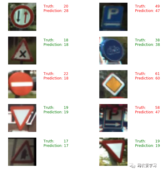
The number after truth in the figure above is the real label, and the number after Prediction is the predicted label.
The current classification test is still the pictures in the training set, so I don't know how the model performs on the unknown data set.
Next, evaluate on the test set.

Model evaluation-verify the accuracy on the test set

The visualization results are very intuitive, but a more precise method is needed to measure the accuracy of the model. This is where the validation set comes into play.

# 加载测试集图片
test_images, test_labels = load_data(test_data_dir)

# 转换图片尺寸
test_images32 = [skimage.transform.resize(image, (32, 32))
                 for image in test_images]
#显示转换后的图片
display_images_and_labels(test_images32, test_labels)

# Run predictions against the full test set.
predicted = session.run([predicted_labels], 
                        feed_dict={images_ph: test_images32})[0]
# 计算准确度
match_count = sum([int(y == y_) for y, y_ in zip(test_labels, predicted)])
accuracy = match_count / len(test_labels)
# 输出测试集上的准确度
print("Accuracy: {:.3f}".format(accuracy))

Accuracy: 0.534

# Close the session. This will destroy the trained model.
session.close()