Big data development-Spark-understand common RDDs in one article

1. Five basic properties

• A list of partitions

• A function for computing each split

• A list of dependencies on other RDDs

• Optionally, a Partitioner for key-value RDDs (e.g. to say that the RDD is hash-partitioned)

• Optionally, a list of preferred locations to compute each split on (e.g. block locations for an HDFS file)

This is written in the comments in the source code of the RDD, the five characteristic attributes are introduced below

1.1 Partition

A partition is the basic unit of the data set. For RDD, each shard will be processed by a computing task and determine the granularity of parallel computing. The user can specify the number of RDD fragments when creating the RDD, if not specified, then the default value will be used

1.2 Calculated function

A function for calculating partition data. The calculation of RDD in Spark is based on shards, and each RDD will implement the compute function to achieve this goal. The compute function combines the iterators and does not need to save the results of each calculation

1.3 Dependency

There are dependencies between RDDs. Each conversion of RDD will generate a new RDD, and the front and back dependencies (lineage) similar to the pipeline are formed between RDDs. When part of the partition data is lost, Spark can recalculate the lost partition data through this dependency, instead of recalculating all partitions of the RDD

1.4 Partitioner

For key-valuethe RDD, the possible partition device ( Partitioner). Spark implements two types of fragmentation functions, one is hash-based HashPartitionerand the other is RangePartitioner based on range. Only key-value RDDs are possible Partitioner, and the value of non-key-value RDDs Parititioneris None. PartitionerThe function determines the RDDnumber of its own shards, and also determines the parent RDD Shufflenumber of shards when outputting

1.5 Priority storage location

A list that stores each Partitionpreferred location (preferred location). For a HDFSfile, this list saves the Partitionlocation of each block. According to the concept of "moving data and not computing", Sparkwhen task scheduling, the computing task will be allocated to the storage location of the data block to be processed as much as possible

2. Common operators between RDD conversions

Starting from the previous RDDbasic features, the programs that are often written in work are creation RDD, RDDconversion, RDDexecution of operators, creation of necessary steps for data corresponding to external systems to flow into the Spark cluster, as for data created from collections , Is generally used in testing, so I won’t go into details. RDDThe conversion corresponds to a special operator called Transformationlazy loading, and the action corresponds to Transformationthe operation that triggers the execution, usually output to the collection, or print out, or return a Value, in addition, is output from the cluster to other systems, which has a professional term Action.

2.1 Common conversion operators

The conversion operator, that is, the conversion operation from one RDD to another RDD, corresponds to some built-in Compute functions, but these functions are divided into wide-dependent operators and narrow-dependent operators with or without shuffle

2.1.1 The difference between wide dependence and narrow dependence

Generally, there are two kinds of articles on the Internet. One is the definition of transportation, that is, whether a parent RDDpartition will be dependent on multiple child partitions. The other is to see if there is any Shuffle, if there Shuffleis a wide dependency, if there is no, it is a narrow dependency. The first is still dependent. Spectral points, the second is to take itself as its own, so it has no reference value. 2.1.3 How to distinguish between wide dependence and narrow dependence, you can look at this between

2.1.2 Common operators for wide and narrow dependencies

Narrow dependency common operators

map(func): Use func for each element in the data set, and then return a new RDD filter(func): Use func for each element in the data set, and then return an RDD containing elements that make func true flatMap(func): similar to map, each Input elements are mapped to 0 or more output elements mapPartitions(func): similar to map, but map uses func on each element, and mapPartitions uses func on the entire partition. Assuming an RDD has N elements and M partitions (N >> M), then the function of map will be called N times, and the function in mapPartitions will be called only M times, processing all elements in one partition at a time mapPartitionsWithIndex(func): with mapPartitions Similarly, more information about the index value of the partition

glom(): Form each partition into an array to form a new RDD type RDD[Array[T]] sample(withReplacement, fraction, seed): sampling operator. Use the specified random seed (seed) to randomly sample the data of the number of fractions, withReplacement indicates whether the extracted data is replaced or not, true is the sampling with replacement, and false is the sampling without replacement.

coalesce(numPartitions,false): No shuffle, generally used to reduce partitions

union(otherRDD): Find the union of two RDDs

cartesian(otherRDD):Cartesian Product

zip(otherRDD): Combine two RDDs into a key-value RDD. By default, the number of partitions and elements of the two RDDs are the same, otherwise an exception will be thrown.

The difference between map and mapPartitions map : processing one piece of data mapPartitionsat a time: processing one partition of data at a time, the data can only be released after the partition's data processing is completed. When resources are insufficient, it is easy to lead to OOM. Best practice : When memory resources are sufficient, it is recommended to use mapPartitions, To improve processing efficiency

Wide dependency common operators

groupBy(func): Group according to the return value of the passed function. Put the same key value into an iterator

distinct([numTasks])): After removing the duplicates of the RDD element, return a new RDD. You can pass in the numTasks parameter to change the number of RDD partitions

coalesce(numPartitions, true): With shuffle, whether to increase or decrease partitions, generally use repartition instead

repartition(numPartitions): Increase or decrease the number of partitions, with shuffle

sortBy(func, [ascending], [numTasks]): Use func to process the data and sort the processed results

intersection(otherRDD): Find the intersection of two RDDs

subtract (otherRDD): Find the difference of two RDDs

2.1.3 How to distinguish between wide dependence and narrow dependence

Here I suggest operators that cannot be understood. From Sparkthe historydependency graph, see Stageif there is any division . If it is divided , it is wide dependency, and if it is not divided , it is narrow dependency. Of course, this is a practical approach. You can explain the problem to colleagues or classmates. When it is time, show your codegive it to him, and then give him the dependency graph. Of course, as a paralleler of theory and practice, I will use another method to judge. It starts from understanding the definition. The definition says whether the parent RDD partition is divided by multiple children. Partition dependency, you can think about it from this perspective, is it possible for the data in a single partition of the parent partition to flow to the partition of different child RDDs, for example, think about the distinct operator, or the sortBy operator, global deduplication and global sorting, assuming just At the beginning 1, 2, and 3 are in a partition. After map(x => (x, null)).reduceByKey((x, y) => x).map(_._1)deduplication, although the number of partitions has not changed, the data of each partition must be read by the data of other partitions to know whether to keep it in the end, from the input partition to the output partition. , after the inevitable convergence of restructuring , so there must be shufflea. sortBySimilarly.

2.2 Common action operators

Action triggers Job. A Spark program (Driver program) contains as many Action operators as there are jobs; Typical Action operators: collect / count collect() => sc.runJob() => ... => dagScheduler.runJob( ) => Job is triggered

collect() / collectAsMap() stats / count / mean / stdev / max / min reduce(func) / fold(func) / aggregate(func)

first()：Return the first element in this RDD take(n)：Take the first num elements of the RDD top(n)：According to the default (descending order) or specified sorting rules, return the first num elements. takeSample(withReplacement, num, [seed]): Return sampled data foreach(func) / foreachPartition(func): similar to map and mapPartitions, the difference is that foreach is ActionsaveAsTextFile(path) / saveAsSequenceFile(path) / saveAsObjectFile(path)

3. Common operations of PairRDD

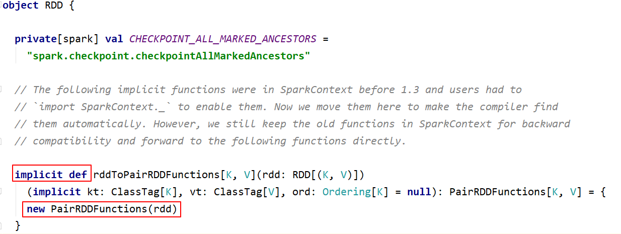
RDD is generally divided into Value type and Key-Value type. The previous introduction is the operation of Value type RDD, the actual use is more key-value type RDD, also known as PairRDD. The operation of Value type RDD is basically concentrated in RDD.scala; the operation of key-value type RDD is concentrated in PairRDDFunctions.scala;

Most of the operators introduced above are valid for Pair RDD. When the value of RDD is key-value, it can be implicitly converted to PairRDD. Pair RDD also has its own Transformation and Action operators;

3.1 Transformation operations of common PairRDD

3.1.1 Similar map operations

mapValues ​​/ flatMapValues ​​/ keys / values, these operations can be implemented using map operations, which are simplified operations.

3.1.2 Aggregation operation [important and difficult]

PariRDD(k, v) has a wide range of applications, aggregate groupByKey / reduceByKey / foldByKey / aggregateByKey combineByKey (OLD) / combineByKeyWithClassTag (NEW) => the underlying implementation subtractByKey: similar to subtract, delete the key in the RDD that is the same as the key in other RDD element

Conclusion : Use the most familiar method for the same efficiency; groupByKey is generally inefficient, so use as little as possible

3.1.3 Sort operation

sortByKey: The sortByKey function acts on PairRDD to sort the Key

3.1.4 join operation

cogroup / join / leftOuterJoin / rightOuterJoin / fullOuterJoin

val rdd1 = sc.makeRDD(Array((1,"Spark"), (2,"Hadoop"), (3,"Kylin"), (4,"Flink")))
val rdd2 = sc.makeRDD(Array((3,"李四"), (4,"王五"), (5,"赵六"), (6,"冯七")))
val rdd3 = rdd1.cogroup(rdd2)
rdd3.collect.foreach(println)
rdd3.filter{case (_, (v1, v2)) => v1.nonEmpty & v2.nonEmpty}.collect
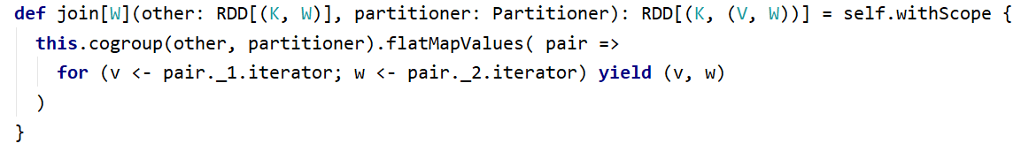
// 仿照源码实现join操作
rdd3.flatMapValues( pair =>
for (v <- pair._1.iterator; w <- pair._2.iterator) yield (v, w)
)
val rdd1 = sc.makeRDD(Array(("1","Spark"),("2","Hadoop"),("3","Scala"),("4","Java")))
val rdd2 = sc.makeRDD(Array(("3","20K"),("4","18K"),("5","25K"),("6","10K")))
rdd1.join(rdd2).collect
rdd1.leftOuterJoin(rdd2).collect
rdd1.rightOuterJoin(rdd2).collect
rdd1.fullOuterJoin(rdd2).collect

3.1.5 Action operation

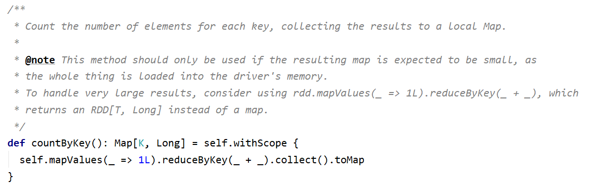
collectAsMap / countByKey / lookup(key)

lookup(key): Efficient search method, only search the data corresponding to the partition (if the RDD has a partitioner)

4. Message

Real knowledge from actual combat, when you want a certain realization, suppose you happen to think of a certain operator, then use it, look at the source code where you don’t understand, and you can do it! Wu Xie, Xiao San Ye, a little rookie in the background, big data, and artificial intelligence. Please pay attention to more