 1. Data characteristics and pain points of the Industrial Internet of Things
The data collection of the Industrial Internet of Things has the characteristics of high frequency, multiple devices, and high dimensions. The amount of data is very large, and there are high requirements for the throughput of the system. At the same time, the industrial Internet of Things often requires the system to be able to process data in real time, to provide early warning, monitoring, and even counter-control to the system. Many systems also need to provide graphical terminals for operators to monitor the operation of equipment in real time, which puts greater pressure on the entire system. For the massive historical data collected, offline modeling and analysis are usually required. Therefore, the data platform of the Industrial Internet of Things has very demanding requirements. It must have very high throughput and low latency; it must be able to process streaming data in real time, and it must be able to process massive amounts of historical data; both To meet the requirements of simple point query, but also to meet the requirements of complex analysis of batch data.
Traditional transactional databases, such as SQL Server, Oracle, and MySQL, cannot meet high-throughput data writing and massive data analysis. Even if the amount of data is small and can meet the requirements of data writing, it cannot respond to requests for real-time computing at the same time.
The Hadoop ecosystem provides multiple components such as messaging engine, real-time data writing, streaming data calculation, offline data warehouse, and offline data calculation. The combination of these big data systems can solve the data platform problem of the Industrial Internet of Things. However, such a scheme is too large and bloated, and the cost of implementation and operation and maintenance is high.
2. Industrial IoT solutions based on time series databases
Take DolphinDB as an example. As a high-performance distributed time series database, DolphinDB database provides a powerful basic platform for data storage and calculation of the Industrial Internet of Things.
- DolphinDB's distributed database can easily support horizontal expansion and vertical expansion, and the throughput and supported data volume of the system can be expanded almost infinitely.
- DolphinDB's stream computing engine supports real-time stream computing processing. The built-in aggregation engine can calculate various aggregation indicators according to the specified time window size and frequency. The aggregation can be either a vertical aggregation on the time axis (from high frequency to low frequency), or a horizontal aggregation of multiple dimensions.
- DolphinDB's in-memory database can support fast data writing, query and calculation. For example, the results of the aggregation engine can be output to a memory table and receive second-level polling instructions from front-end BI (such as Grafana).
- DolphinDB integrates database, distributed computing, and programming language, and can quickly complete complex distributed computing, such as regression and classification, in the library. This greatly accelerates the offline analysis and modeling of massive historical data.
- DolphinDB also implements interfaces with some open source or commercial BI tools. It is convenient for users to visualize or monitor equipment data.
3. Case summary
There are a total of 1,000 sensing devices in the production workshop of the enterprise, and each device collects data every 10ms. To simplify the demo script, it is assumed that the collected data has only three dimensions, all of which are temperature. The tasks to be completed include:
- Store the collected raw data in the database. Offline data modeling needs to use these historical data.
- The average temperature index of each device in the past minute is calculated in real time, and the calculation frequency is performed every two seconds.
- Because the operator of the equipment needs to grasp the temperature change in the fastest time, the front-end display interface queries the results of real-time calculations every second and refreshes the temperature change trend graph.
4. Case implementation
4.1 The functional module design of the system
For the above case, we first need to enable the distributed database of DolphinDB and create a distributed database named iotDemoDB to save the collected real-time data. The database is partitioned in two dimensions: date and device. The date is partitioned by value, and the device is partitioned by range. To clean up expired data in the future, you can simply delete the old date partition.
Enable streaming data publishing and subscription functions. Subscribe to high-frequency data streams for real-time calculations. The createStreamingAggregator function can create an indicator aggregation engine for real-time calculation. In the case, we specify that the calculation window size is 1 minute, calculate the temperature average of the past 1 minute every 2 seconds, and then save the calculation result to the low frequency data table for front-end polling.
Deploy the front-end Grafana platform to display the trend graph of the calculation results, set the DolphinDB Server to poll once every 1 second, and refresh the display interface.
4.2 Server deployment
In this demo, in order to use a distributed database, we need to use a single-machine multi-node cluster. You can refer to the single-machine multi-node cluster deployment guide . Here we have configured a cluster of 1 controller + 1 agent + 4 datanodes. The main configuration files are listed below for reference:
cluster.nodes:
localSite,mode
localhost:8701:agent1,agent
localhost:8081:node1,datanode
localhost:8083:node2,datanode
localhost:8082:node3,datanode
localhost:8084:node4,datanode
Since the DolphinDB system does not enable the Streaming module function by default, we need to enable it by explicitly configuring it in cluster.cfg. Because the amount of data used in this demo is not large, in order to avoid the complexity of the demo, so here only Node1 is enabled for data subscription.
cluster.cfg:
maxMemSize = 2
workerNum=4
persistenceDir = dbcache
maxSubConnections=4
node1.subPort=8085
maxPubConnections=4
In the actual production environment, it is recommended to use a multi-physical machine cluster. You can refer to the multi-physical machine cluster deployment guide .
4.3 Implementation steps
First, we define a sensorTemp flow data table to receive real-time collected temperature data. We use the enableTablePersistence function to persist the sensorTemp table. The maximum amount of data retained in the memory is 1 million rows.
share streamTable(1000000:0,`hardwareId`ts`temp1`temp2`temp3,[INT,TIMESTAMP,DOUBLE,DOUBLE,DOUBLE]) as sensorTemp
enableTablePersistence(sensorTemp, true, false, 1000000)
By subscribing to the streaming data table sensorTmp, the collected data is saved in a distributed database in quasi-real-time batches. The distributed table uses two partition dimensions: date and device number. In the big data scenario of the Internet of Things, obsolete data is often cleared, so that the partition mode can quickly clear the expired data simply by deleting the partition on the specified date. The last two parameters of the subscribeTable function control the frequency of data storage. Only when the subscription data reaches 1 million or the time interval reaches 10 seconds will the data be written to the distributed database in batches.
db1 = database("",VALUE,2018.08.14..2018.12.20)
db2 = database("",RANGE,0..10*100)
db = database("dfs://iotDemoDB",COMPO,[db1,db2])
dfsTable = db.createPartitionedTable(sensorTemp,"sensorTemp",`ts`hardwareId)
subscribeTable(, "sensorTemp", "save_to_db", -1, append!{dfsTable}, true, 1000000, 10)
While the streaming data is stored in a distributed database, the system uses the createStreamAggregator function to create an indicator aggregation engine for real-time calculation. The first parameter of the function specifies the window size as 60 seconds, the second parameter specifies the average operation every 2 seconds, and the third parameter is the meta code of the operation. The calculation function can be specified by the user, any system supports Or user-defined aggregation functions can be supported here. By specifying the grouping field hardwareId, the function will divide the stream data into 1000 queues by device for average calculation, and each device will calculate the corresponding average temperature according to its own window. Finally, subscribe to the stream data through subscribeTable, trigger real-time calculation when new data comes in, and save the result of the operation to a new data stream table sensorTempAvg.
createStreamAggregator parameter description: window time, operation interval time, aggregation operand code, raw data input table, operation result output table, time series field, group field, threshold of the number of trigger GC records.
share streamTable(1000000:0, `time`hardwareId`tempavg1`tempavg2`tempavg3, [TIMESTAMP,INT,DOUBLE,DOUBLE,DOUBLE]) as sensorTempAvg
metrics = createStreamAggregator(60000,2000,<[avg(temp1),avg(temp2),avg(temp3)]>,sensorTemp,sensorTempAvg,`ts,`hardwareId,2000)
subscribeTable(, "sensorTemp", "metric_engine", -1, append!{metrics},true)
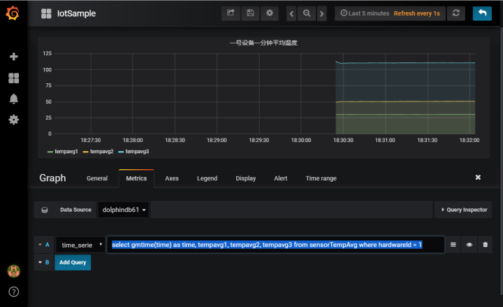
When DolphinDB Server saves and analyzes high-frequency data streams, the Grafana front-end program polls the results of real-time calculations every second and refreshes the trend graph of the average temperature. DolphinDB provides a datasource plugin for Grafana_DolphinDB. For Grafana installation and DolphinDB plugin configuration, please refer to the Grafana configuration tutorial .
After completing the basic configuration of grafana, add a Graph Panel, enter in the Metrics tab:
select gmtime(time) as time, tempavg1, tempavg2, tempavg3 from sensorTempAvg where hardwareId = 1
This script is to select the average temperature table obtained by real-time calculation of the No. 1 device.
Finally, start the data simulation generation program to generate simulated temperature data and write it into the stream data table.
Data scale: 1000 devices, 3 dimensions per point, 10ms frequency to generate data, 8 bytes per dimension (Double type) calculation, data flow rate is 24Mbps, lasting 100 seconds.
def writeData(){
	hardwareNumber = 1000
	for (i in 0:10000) {
		data = table(take(1..hardwareNumber,hardwareNumber) as hardwareId ,take(now(),hardwareNumber) as ts,rand(20..41,hardwareNumber) as temp1,rand(30..71,hardwareNumber) as temp2,rand(70..151,hardwareNumber) as temp3)
		sensorTemp.append!(data)
		sleep(10)
	}
}
submitJob("simulateData", "simulate sensor data", writeData)
Click here to download the complete demo script.