Deep learning from scratch-neural network (four), two classification problems, IMDB data set use

IMDB data set

Internet movie data contains 50,000 severely polarized comments. Positive and negative comments each account for 50%.
The data set is also built into the Keras library.

The comment data has been preprocessed, and the comments (words) are converted into a sequence of integers, and each integer corresponds to a word in the dictionary.

Load data set

from keras.datasets import imdb

(train_data,train_labels),(test_data,test_labels) = imdb.load_data(num_words=10000)
#第一条评论的单词索引列表
print(train_data[0])
#1表示正面品论，0表示负面评论
print(train_labels[0])
#取所有测试单词所有的最大的索引值
print(max([max(sequence) for sequence in train_data]))

num_words=10000 is to take the most frequently occurring 10000 words and discard low-frequency words. Reduce the amount of vector data.
Both train_data and test_data are lists of reviews (consisting of word indexes).
Both train_labels and test_labels are lists of 0 and 1.
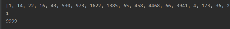You can see that the maximum 9999 means that the index does not exceed 10000

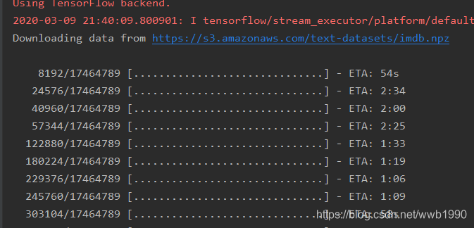
The dataset will be downloaded the first time it is loaded

Decode to english

#某条评论解码为英文
word_index = imdb.get_word_index()
reverse_word_index = dict(
    [(value,key) for (key,value) in word_index.items()]
)
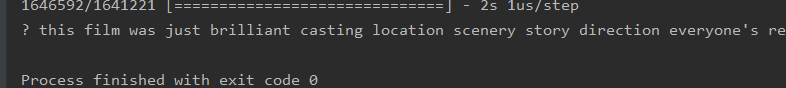
decoded_review = ' '.join(
    [reverse_word_index.get(i-3,'?') for i in train_data[0]]
)
print(decoded_review)

imdb.get_word_index() is a dictionary of word mapping integers, and its key value is reversed to look up words according to the index.
Where i-3 is because 0, 1, and 2 are the index reserved for padding, sequence start, unknown word

Data processing

import numpy as np

#转换为10000维的向量，索引的位置是1，其他位置是0
def vectorize_sequences(sequences,dimension=10000):
    results = np.zeros((len(sequences),dimension))
    for i, sequence in enumerate(sequences):
        results[i,sequence] = 1.
    return results
#数据向量化
x_train = vectorize_sequences(train_data)
x_test = vectorize_sequences(test_data)
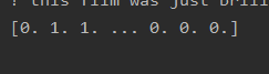
print(x_train[0])
#标签向量化
y_train = np.asarray(train_labels).astype('float32')
y_test = np.asarray(test_labels).astype('float32')

Convert the index value of each comment to a 10,000-dimensional vector. The index value is set to 1, and the remaining positions are set to 0.
For example, if a comment is [1,3,5], it becomes [0,1,0,1,0,1,0,0,0,0 …,0].

Build a network

from keras import models
from keras import layers

#模型定义
model = models.Sequential()
model.add(layers.Dense(16,activation='relu',input_shape=(10000,)))
model.add(layers.Dense(16,activation='relu'))
model.add(layers.Dense(1,activation='sigmoid'))
#定义优化器，损失函数，指标
model.compile(optimizer='rmsprop',
              loss='binary_crossentropy',
              metrics=['accuracy'])

The model has three layers.

• The first and second layers have 16 hidden units, and a 10,000-dimensional vector is input. In addition to the tensor operation, relu is one of the activation functions, which turns the linear transformation set into nonlinear.
• The third layer outputs 1 dimension, and sigmod is the probability of normalizing the output to [0,1].

For two classification problems, the output is a probability value (the probability of a positive evaluation).
Thus the choice of cross-entropy (crossentropy) calculated loss.
The optimizer uses rmsprop. This is the best example summarized by the predecessor. As for why I chose these two, I will study in the following chapters.

Validation set

In order to monitor the accuracy of the model on unseen data during the training process, 10,000 samples were taken from the data to be used as a validation set.

#取10000用于验证集
x_val = x_train[:10000] #验证集
partial_x_train = x_train[10000:]

y_val = y_train[:10000] #验证集
partial_y_trail = y_train[10000:]

Training model

#训练模型
history = model.fit(partial_x_train,
                    partial_y_trail,
                    epochs=20,
                    batch_size=512,
                    validation_data=(x_val,y_val))
                    
history_dict = history.history
print(history_dict.keys())

We input the training data set partial_x_train and the training tag set partial_y_trail.
Training times of all data*20.
Fetch 512 pieces of data at a time.
The history contains all the data in the training process.
validation_data is the validation set taken out in the previous step.

History contains all the data in the training process. Print the metrics contained in history_dict.

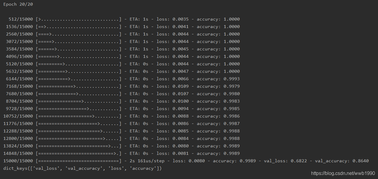
You can see that it includes verification accuracy, training accuracy, verification loss, and training loss.

Let's use matplot to plot the trend of these indicators:

Loss change graph:

loss_values = history_dict['loss']
val_loss_values = history_dict['val_loss']

epochs = range(1,len(loss_values)+1)

plt.plot(epochs,loss_values,'bo',label='Training loss') #bo是蓝色圆点
plt.plot(epochs,val_loss_values,'b',label='Validation loss') #b是蓝色实线
plt.title('Training and validation loss')
plt.xlabel('Epochs')
plt.ylabel('Loss')
plt.legend()
plt.show()

Accuracy change chart:

plt.clf() #清空图表

acc_values = history_dict['acc']
val_acc_values  = history_dict['val_acc']

plt.plot(epochs,acc_values,'bo',label='Training acc') #bo是蓝色圆点
plt.plot(epochs,val_acc_values,'b',label='Validation acc') #b是蓝色实线
plt.title('Training and validation accuracy')
plt.xlabel('Epochs')
plt.ylabel('Accuracy')
plt.legend()
plt.show()

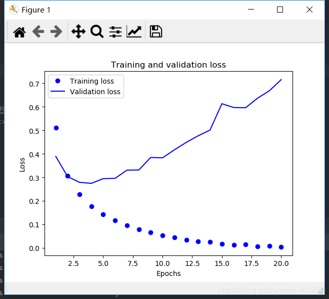
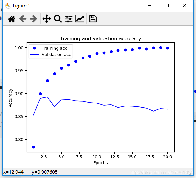It can be seen that the training loss continues to decrease and the training accuracy continues to increase. This meets the optimization expectations of gradient descent.
But you can see the verification loss and verification accuracy . It can be seen from the figure that they reached the best in the third to fourth cycles.

In short, the performance has improved on the training data, but the performance has changed on the validation data that has not been seen. This is overfitting .
After the second round, the training data is over-optimized, and the final learning result is only for the training data. Data outside the training set cannot be spread.

A solution to reduce overfitting is needed. Come to learn in later chapters.

A rough and simple scheme is used here.
We only train for four rounds.
Modify the training parameter epochs=4

#训练模型
history = model.fit(partial_x_train,
                    partial_y_trail,
                    epochs=4,
                    batch_size=512,
                    validation_data=(x_val,y_val))

Add the test code of the test set after calling fit() to train, and output the result:

result = model.evaluate(x_test,y_test)
print(result)

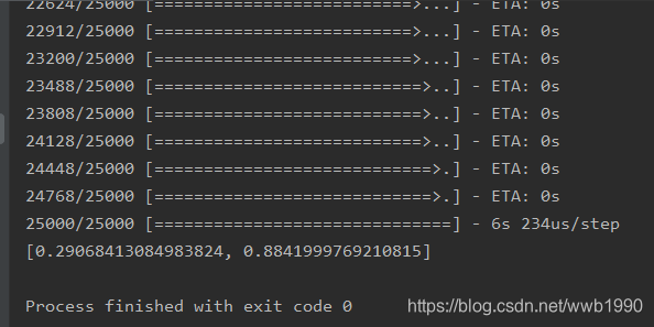
It can be seen that this rough strategy achieves an accuracy of 88%. Later, we will study strategies to better reduce overfitting and do more training.

The trained network uses predict to predict the probability of a positive review.

predictResult = model.predict(x_test)
print(predictResult)

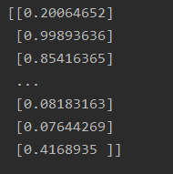
It can be seen that there are very certain (>0.99 or <0.01) and some uncertain (0.4~0.6).

This is the end of this section. Then you can try it yourself
1. Use 1 or 3 hidden layers
2. Replace the hidden units with 32 or 64
3. Use the loss function mse
4. Use the activation function tanh

Integrate all the above codes: (modify the number of epochs by yourself)

from keras.datasets import imdb
import numpy as np
from keras import models
from keras import layers
import matplotlib.pyplot as plt

(train_data,train_labels),(test_data,test_labels) = imdb.load_data(num_words=10000)
# #第一条评论的单词索引列表
# print(train_data[0])
# #1表示正面品论，0表示负面评论
# print(train_labels[0])
# #取所有测试单词所有的最大的索引值
# print(max([max(sequence) for sequence in train_data]))

# #某条评论解码为英文
# word_index = imdb.get_word_index()
# reverse_word_index = dict(
#     [(value,key) for (key,value) in word_index.items()]
# )
# decoded_review = ' '.join(
#     [reverse_word_index.get(i-3,'?') for i in train_data[0]]
# )
# print(decoded_review)

#转换为10000维的向量，索引的位置是1，其他位置是0
def vectorize_sequences(sequences,dimension=10000):
    results = np.zeros((len(sequences),dimension))
    for i, sequence in enumerate(sequences):
        results[i,sequence] = 1.
    return results
#数据向量化
x_train = vectorize_sequences(train_data)
x_test = vectorize_sequences(test_data)
print(x_train[0])
#标签向量化
y_train = np.asarray(train_labels).astype('float32')
y_test = np.asarray(test_labels).astype('float32')

#模型定义
model = models.Sequential()
model.add(layers.Dense(16,activation='relu',input_shape=(10000,)))
model.add(layers.Dense(16,activation='relu'))
model.add(layers.Dense(1,activation='sigmoid'))
#定义优化器，损失函数，指标
model.compile(optimizer='rmsprop',
              loss='binary_crossentropy',
              metrics=['accuracy'])

#取10000用于验证集
x_val = x_train[:10000] #验证集
partial_x_train = x_train[10000:]

y_val = y_train[:10000] #验证集
partial_y_trail = y_train[10000:]

#训练模型
history = model.fit(partial_x_train,
                    partial_y_trail,
                    epochs=4,
                    batch_size=512,
                    validation_data=(x_val,y_val))

history_dict = history.history
print(history_dict.keys())

loss_values = history_dict['loss']
val_loss_values = history_dict['val_loss']

epochs = range(1,len(loss_values)+1)

plt.plot(epochs,loss_values,'bo',label='Training loss') #bo是蓝色圆点
plt.plot(epochs,val_loss_values,'b',label='Validation loss') #b是蓝色实线
plt.title('Training and validation loss')
plt.xlabel('Epochs')
plt.ylabel('Loss')
plt.legend()
plt.show()

plt.clf() #清空图表

acc_values = history_dict['accuracy']
val_acc_values  = history_dict['val_accuracy']

plt.plot(epochs,acc_values,'bo',label='Training acc') #bo是蓝色圆点
plt.plot(epochs,val_acc_values,'b',label='Validation acc') #b是蓝色实线
plt.title('Training and validation accuracy')
plt.xlabel('Epochs')
plt.ylabel('Accuracy')
plt.legend()
plt.show()

result = model.evaluate(x_test,y_test)
print(result)

predictResult = model.predict(x_test)
print(predictResult)