Task2: Data exploratory analysis (EDA)
- What is EDA
- EDA goals
- The main work
- Import and observe data
- Data overview
- Relevant statistics
- type of data
- Data detection
- Missing value detection
- Outlier detection
- Forecast distribution
- General distribution overview (unbounded Johnson distribution, etc.)
- View skewness and kurtosis
- Check the specific frequency of the predicted value
- Characteristics
- Category characteristics
- unique distribution
- Visualization
- Box plot
- Violin illustration
- Bar chart
- Visualize the feature frequency of each category
- Digital features
- Correlation analysis
- Feature skewness and peak
- Digital feature distribution visualization
- Visualization of digital features
- Visualization of multivariate mutual regression relationship
What is EDA
Exploratory Data Analysis (EDA) refers to the exploration of existing data (especially the original data obtained from investigations or observations) with as few a priori assumptions as possible , through mapping, tabulation, A data analysis method that explores the structure and laws of data by means of equation fitting and calculation of feature quantities . Especially when we are faced with all kinds of messy "dirty data", we are often at a loss and don't know where to start to understand the data currently in hand, exploratory data analysis is very effective. Exploratory data analysis was proposed in the 1960s, and its method was proposed by American statistician John Tukey.
- Qualitative data: Descriptive nature
a) Classification: Classification by name-blood type, city
b) Sequence: Ordered classification-performance (ABC) - Quantitative data: describe the quantity
a) fixed distance: can add and subtract-temperature, date
b) fixed ratio: can multiply and divide-price, weight
Check the Tianchi documentation to see the practical significance of the data.
| Field | Description |
|---|---|
| SaleID | Transaction ID, unique code |
| name | Automobile transaction name, desensitized |
| regDate | Car registration date, such as 20160101, January 1, 2016 |
| model | Model code, desensitized |
| brand | Car brand, desensitized |
| bodyType | Body type: luxury car: 0, mini car: 1, van: 2, bus: 3, convertible: 4, two-door car: 5, commercial vehicle: 6, mixer truck: 7 |
| fuelType | Fuel type: gasoline: 0, diesel: 1, liquefied petroleum gas: 2, natural gas: 3, hybrid: 4, other: 5, electric: 6 |
| gearbox | Transmission: manual: 0, automatic: 1 |
| power | Engine power: range [0, 600] |
| kilometer | The car has traveled kilometers, the unit is ten thousand kilometers |
| notRepairedDamage | The car has unrepaired damage: Yes: 0, No: 1 |
| regionCode | Area code, desensitized |
| seller | Seller: Individual: 0, Non-individual: 1 |
| offerType | Quotation Type: Offer: 0, Request: 1 |
| creatDate | When the car goes online, that is, when it starts to sell |
| price | Used car transaction price (forecast target) |
| v series features | Anonymous features, 15 anonymous features including v0-14 |
EDA goals
1. Understand the data set and make preliminary analysis;
2. Understand the relationship between the variables in the comparison data set;
3. Data processing/feature engineering;
4. Make a graphic summary of the data set and analyze the correlation between features and labels.
Exploratory analysis steps
- Form hypotheses, determine themes to explore
- Clean up data, deal with dirty data
- Evaluate the quality of the data, you can weight the data of different quality
- data report
- Explore and analyze each variable
- Explore the relationship between each independent variable and the dependent variable
- Explore the correlation between each independent variable
- Analyze data from different dimensions
The main work
Import and observe data
Import related libraries
import warnings
warnings.filterwarnings('ignore')
# 避免出现:代码正常运行,但提示警告

import pandas as pd
import numpy as np
import matplotlib.pyplot as plt
import seaborn as sns
import missingno as msno
## 通过Pandas载入数据
Train_data = pd.read_csv('datalab/231784/used_car_train_20200313.csv', sep=' ')
Test_data = pd.read_csv('datalab/231784/used_car_testA_20200313.csv', sep=' ')
# 源文件指定为' '分隔符,以防报错
Train_data.head(3).append(Train_data.tail(3))
# 查看训练集前3行和后3行的数据,结果略
Train_data.shape # 输出:(150000, 31)
Test_data.shape # 输出:(50000, 30)
# 训练集比测试集多1列:'price'
Train_data.describe()
# 通过describe查看相关统计量,掌握数据的大概范围以及对异常值的判断
Train_data.info()
# 熟悉数据类型,其中'notRepairedDamage'是object类型,其余都是数值
Train_data.isnull().sum()
# 查看每个字段的缺失情况(汇总)

About missing values :
1. If the number of missing values is small, generally choose to fill;
2. If you use tree models such as lgb, you can directly vacate, let the tree optimize by itself;
3. If there are too many nans , you can delete them.
Train_data['notRepairedDamage'].value_counts()
# 对'notRepairedDamage'的值类型进行计数
# 输出:0.0    111361
#      -       24324
#      1.0     14315

Train_data['notRepairedDamage'].replace('-', np.nan, inplace=True)
# 将‘ - ’替换成nan
Among them, we found that the "seller" and "offerType" features are severely skewed and generally will not help predictions, so we delete them first:
Train_data["seller"].value_counts()
Train_data["offerType"].value_counts()
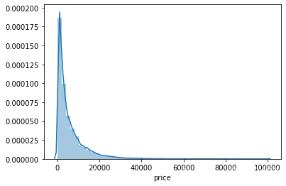
View the distribution of the predicted value'price':
# 查看偏度和峰度
sns.distplot(Train_data['price']);
print("Skewness: %f" % Train_data['price'].skew())
print("Kurtosis: %f" % Train_data['price'].kurt())
# 输出:Skewness: 3.346487
#      Kurtosis: 18.995183
Plot the probability distribution of the skewness and kurtosis of each variable in the training set:
sns.distplot(Train_data.skew(),color='blue',axlabel ='Skewness')
sns.distplot(Train_data.kurt(),color='orange',axlabel ='Kurtness')


# 查看预测值price的具体频数
plt.hist(Train_data['price'], orientation = 'vertical',histtype = 'bar', color ='red')
plt.title( 'price')
plt.show()

The distribution after logarithmic transformation is more uniform:
plt.hist(np.log(Train_data['price']), orientation = 'vertical',histtype = 'bar', color ='red')
plt.title( 'log-price')
plt.show()

1. Category characteristics
categorical_features = ['name', 'model', 'brand', 'bodyType', 'fuelType', 'gearbox', 'notRepairedDamage', 'regionCode',]
2. Digital features
numeric_features = ['power', 'kilometer', 'v_0', 'v_1', 'v_2', 'v_3', 'v_4', 'v_5', 'v_6', 'v_7', 'v_8', 'v_9', 'v_10', 'v_11', 'v_12', 'v_13','v_14' ]
3. Feature nunique distribution
# 特征nunique分布
for cat_fea in categorical_features:
    print(cat_fea + "的特征分布如下:")
    print("{}特征有{}个不同的值".format(cat_fea, Train_data[cat_fea].nunique()))
    print(Train_data[cat_fea].value_counts())
result:
name特征有99662个不同的值
model特征有248个不同的值
brand特征有40个不同的值
bodyType特征有8个不同的值
fuelType特征有7个不同的值
gearbox特征有2个不同的值
notRepairedDamage特征有2个不同的值
regionCode特征有7905个不同的值
View the category feature distribution of the training set:
for cat_fea in categorical_features:
    print(cat_fea + "的特征分布如下:")
    print("{}特征有个{}不同的值".format(cat_fea, Train_data[cat_fea].nunique()))
    print(Train_data[cat_fea].value_counts())
Relevance visualization:
price_numeric = Train_data[numeric_features]
correlation = price_numeric.corr()

f , ax = plt.subplots(figsize = (7, 7))
plt.title('Correlation of Numeric Features with Price',y=1,size=16)
sns.heatmap(correlation,square = True,  vmax=0.8)

Visualization of the distribution of various digital features:
f = pd.melt(Train_data, value_vars=numeric_features)
g = sns.FacetGrid(f, col="variable",  col_wrap=2, sharex=False, sharey=False)
g = g.map(sns.distplot, "value")
Visualization of the relationship between various digital features:
sns.set()
columns = ['price', 'v_12', 'v_8' , 'v_0', 'power', 'v_5',  'v_2', 'v_6', 'v_1', 'v_14']
sns.pairplot(Train_data[columns],size = 2 ,kind ='scatter',diag_kind='kde')
plt.show()
Generate a data preview report:
Use pandas_profiling to generate data reports
Use pandas_profiling to generate a more comprehensive visualization and data report (relatively simple and convenient) and finally open the html file
import pandas_profiling
pfr = pandas_profiling.ProfileReport(Train_data)
pfr.to_file("./example.html")