PyFR Getting Started Guide

The Flux Reconstruction (FR) format is a high-precision compact fluid numerical format. PyFR is an open source CFD package that uses a very accurate FR format to deal with some of the most challenging fluid flow problems in the world. Especially when it comes to uneven turbulence. Related blogs can be found on the Nvidia blog . PyFR's official website offers downloads and manuals on. This article is an introductory guide based on the above content, the operating platform is Ubuntu 19.10.

installation

1. Install basic dependencies, the command is

sudo pip3 install xxx

These xxxinclude:

appdirs >= 1.4.0
gimmik >= 2.0
h5py >= 2.6
mako >= 1.0.0
mpi4py >= 2.0
numpy >= 1.8
pytools >= 2016.2.1

2. Check the gcc version:, gcc --versionit should be no less than 4.9.
3. Install the remaining dependencies:

sudo apt install python3 python3-pip libopenmpi-dev openmpi-bin
sudo apt install metis libmetis-dev libblas3
pip3 install virtualenv

4. Install paraview:sudo apt install paraview
5. Set up the virtual environment:

python3 -m virtualenv ENV3
source ENV3/bin/activate

And install PyFR in the virtual environment:pip install pyfr

Run command

PyFR uses three file formats:

• .ini——Parameter file
• .pyfrm——Grid file
• .pyfrs-Solution file

PyFR provides several commands:

• pyfr import——Import .msh or .pyfrm format files, which contain grid information. E.g:pyfr import mesh.msh mesh.pyfrm
• pyfr partition-Divide the existing grid and its related solution files. E.g:pyfr partition 2 mesh.pyfrm solution.pyfrs .
• pyfr run-Run a simulation. E.g:pyfr run mesh.pyfrm configuration.ini
• pyfr restart——Restart a simulation based on the existing solution file. E.g:pyfr restart mesh.pyfrm solution.pyfrs
• pyfr export- The .pyfrsfile conversion nonstructural VTK .vtuor pvtufile.

To run PyFR in parallel, pyfruse the prefix before the command mpiexec -n <cores/devices>. Note that the grid should be divided in advance, and the number of cores or devices must be equal to the number of partitions. Then pyfr runadd parallel parameters at the end: -b cuda-Cuda parallel, -b openmp-OpenMP parallel, -b opencl-OpenCL parallel. If the previous operations are correct, you should be able to use OpenMP directly at this time. Cuda and OpenCL need to be installed by themselves.

Example: Two-dimensional Euler vortex

Take OpenMP as an example. Download the source code from the PyFR website, and examplescopy the folder into a suitable working directory. euler_vortex_2dOpen the terminal in the folder.

1. First, start the python virtual environment:source ~/ENV3/bin/activate
2. Convert the mesh file:pyfr import euler_vortex_2d.msh euler_vortex_2d.pyfrm
3. Split the grid into two partitions:pyfr partition 2 euler_vortex_2d.pyfrm .
4. Run: mpiexec -n 2 pyfr run -b openmp -p euler_vortex_2d.pyfrm euler_vortex_2d.ini
   (Note: The parallel parameter here is the -b openmporiginal text of the manual -b cuda. It -n 2corresponds to the two partitions in step 3.)
5. Convert the last frame of data into a .vtuformat file. The command is: pyfr export euler_vortex_2d.pyfrm euler_vortex_2d-100.0.pyfrs euler_vortex_2d-100.0.vtu -d 4
   There are two points to explain in this command: one is to bring the .pyfrm file, and the other is to use the last parameter -d 4, which means to subdivide the unit into 4 linear subunits to improve the display accuracy.
6. Open the .vtufile with Paraview . The velocity field is as follows: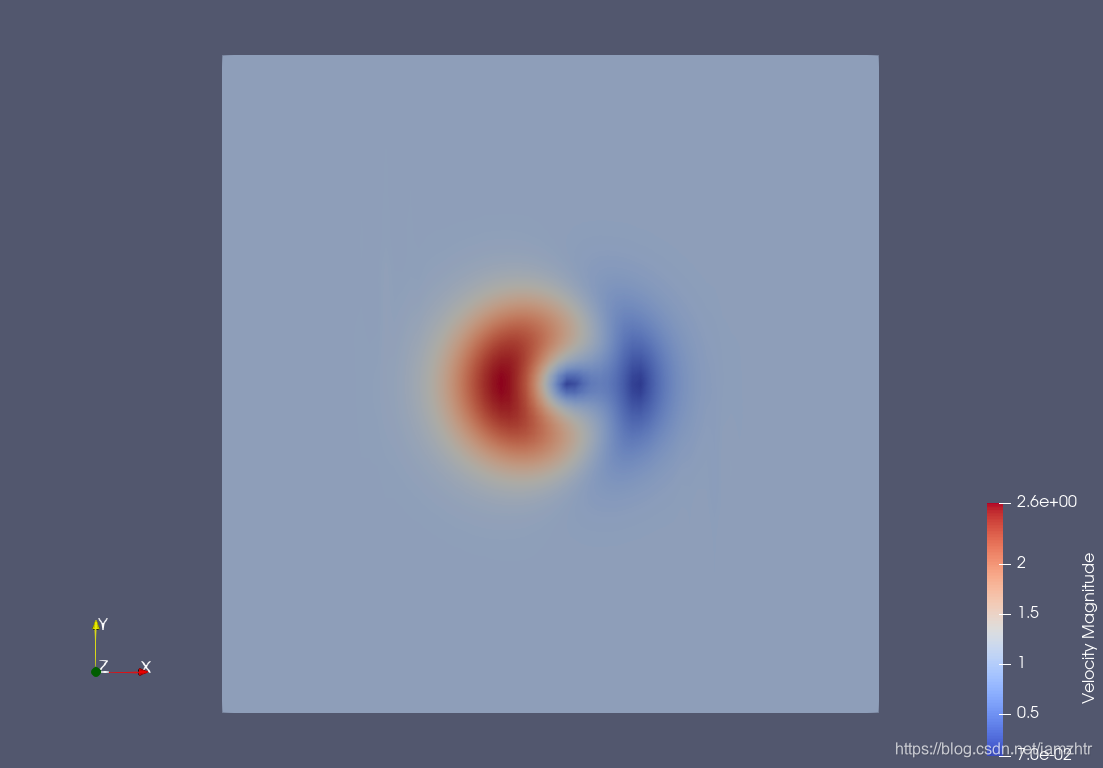

postscript

In particular, it should be pointed out that from the above calculation examples, the nspeed is the fastest when the number of parallel threads using OpenMP is exactly equal to the number of physical cores of the computer, otherwise it will slow down sharply. For example, on my laptop, the -n 2running time is only 19 seconds, -n 4or a single thread takes a few hours. To be honest, I didn't understand why the difference was so big.