Article Directory
- Class Q & A
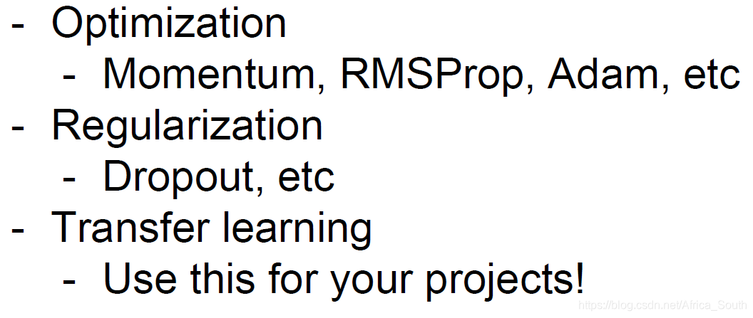
- 1. Better optimization (Fancier optimization)
- 1.1 SGD optimization
- 1.2 Momentum-based SGD
- 1.3 AdaGrad
- 1.4 Adam
- 1.5 Choice of learning rate
- 1.6 Second-Order Optimization (Second-Order Optimization)
- 1.7 Model integration
- 2. Regularization (Regularization)
- 3. Transfer Learning
- to sum up
- References
Class Q & A
- A0: The following comparison of optimization algorithms should be based on convex optimization.
- Q1: How can SGD with momentum handle bad gradient directions?
- Q2: Where is the Dropout layer used?
- A2: Generally, adding DP after the fully connected layer inactivates some neurons. Of course, it can also be added after the convolution layer, but the specific method makes the activation map (activation map) obtained by part of the convolution kernel to 0.
- Q3: What effect does Dropout have on the gradient return?
- A3: Dropout makes gradient feedback only happen to some neurons, which makes our training slower, but the final robustness is better.
- Q4: In general, how many regularization methods do we use?
- A4: Normally, we will use BN because it does play a role in regularization. However, we generally do not cross-validate which regularization methods need to be used, but are targeted. When we find that the model is over-fitted, appropriate regularization methods are added.
1. Better optimization (Fancier optimization)
1.1 SGD optimization
Previously, we introduced a simple gradient update algorithm SGD , which is a fixed step size and updates along the direction of the negative gradient:
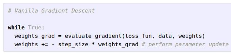
However, it also has some problems.
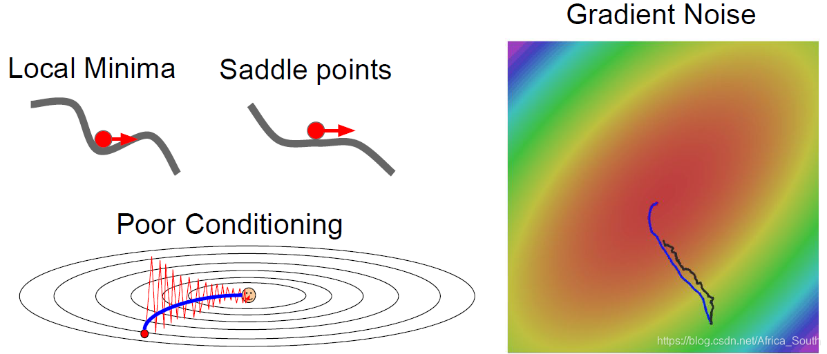
- Suppose we have a loss function L and a two-dimensional weight W, and the loss L is insensitive to changes in one direction (dimension) of W (such as horizontal), and sensitive to changes in another direction (such as vertical). In other words, if it is updated in the vertical direction, our loss will fall faster.
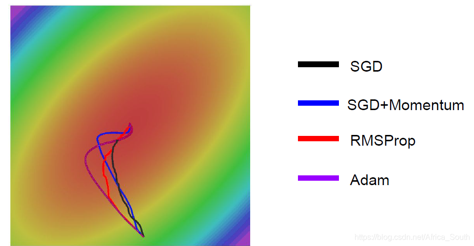
However, the SGD algorithm allows us to update along the combined direction of the two directions. Overall, it will show a zigzag (jitter). As shown in the figure below, the contour line indicates that the loss change along the horizontal direction is very small.
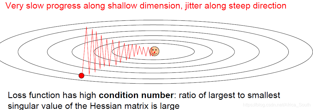
- The above situation is more obvious on a high-dimensional matrix, because the direction of the gradient is more complicated.
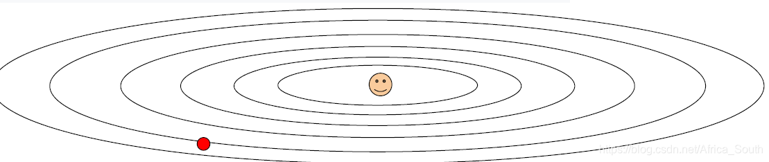
- Relatively easy to fall into local minimum and saddle point
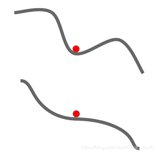
- The local minimum gradient is equal to 0, making the weight almost impossible to update; the gradient near the saddle point is very small, making the weight update very slow (especially in the high-dimensional case, there are many saddle points).
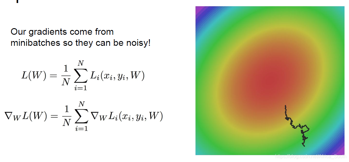
- SGD calculates the gradient on a sample, but when the number of samples is large, our calculation is too large. Therefore, we often use Mini-batch SGD, but such a gradient is an estimated value of a batch, which may introduce noise and make the parameter update more tortuous.
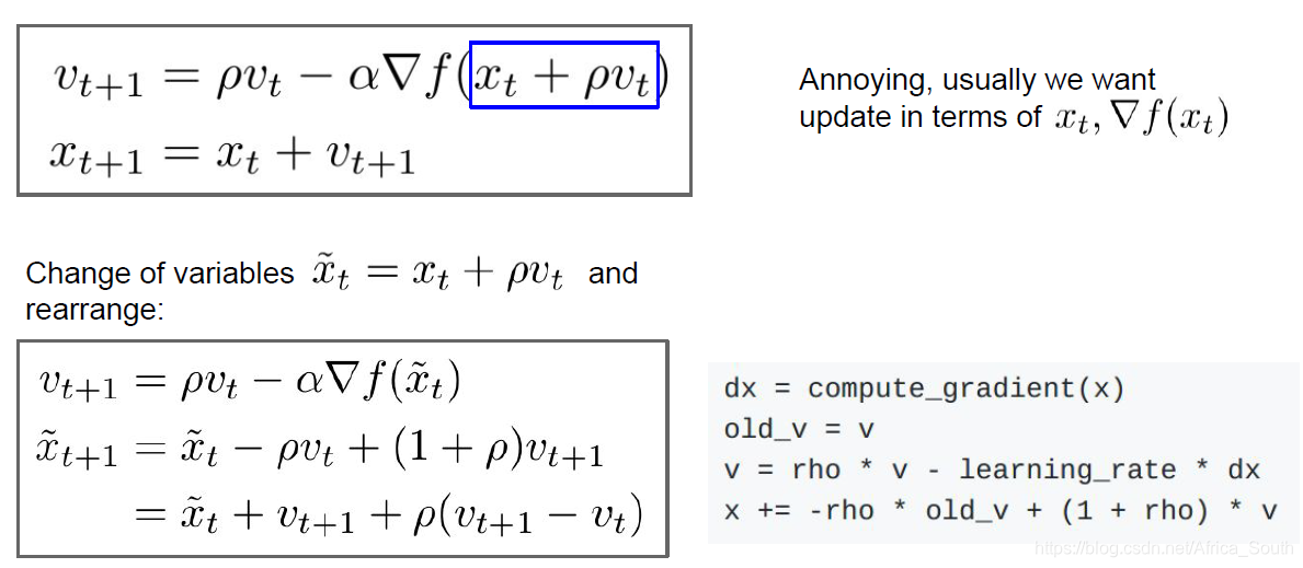
1.2 Momentum-based SGD
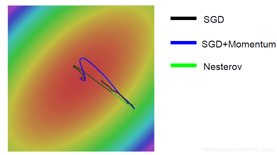
SGD+Momentum
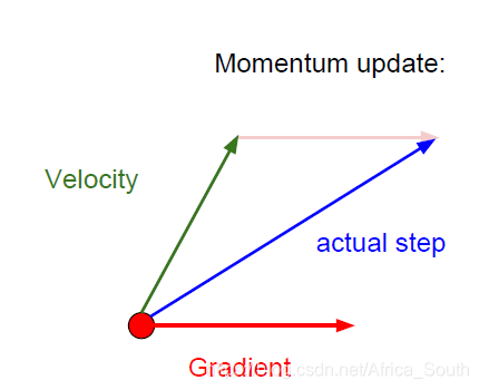
- That is to add a momentum term to our gradient term:
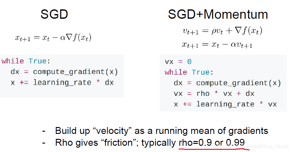
- It makes us still have a certain speed at the local minimum point and saddle point. For the previous zigzag drop, it will accumulate faster in the sensitive direction, and slow down the speed in the less sensitive direction, thus easily offsetting these jitters:
- At the same time, the update direction of momentum is the previous speed + current gradient, which can avoid noise errors to a certain extent.
Nesterov Momentum + SGD
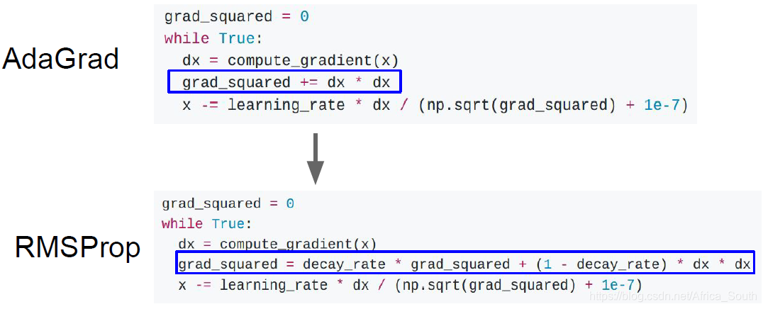
1.3 AdaGrad
- The core is to maintain a training process of gradient square estimate
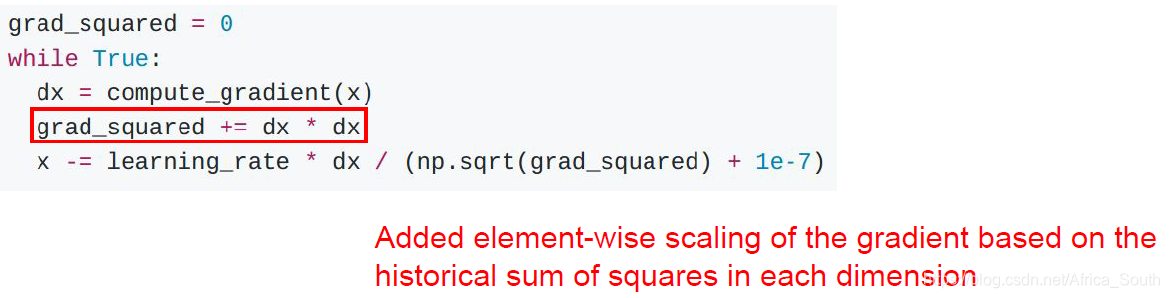
- This accumulation of gradients will slow down the update step size in the direction of the dimension with large gradient, and on the contrary will increase the update step size in the direction of the dimension with small gradient. That is, it will perform similar optimizations in each dimension.
- As our training continues, as the gradient accumulates, the learning step will become smaller and smaller. When the objective function is a convex function, when approaching the extreme point, we move more and more slowly. But for non-convex functions, it may fall into the local best.
Variant-RMSProp
- Like previous momentum, we add in the gradient square to add on a history of decay .
1.4 Adam
- This optimization method is a combination of the first two methods.
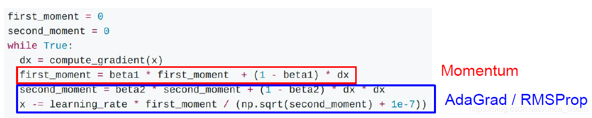
- Q: What happened during the previous updates?
- A: Our weighting factor is generally 0.9 or 0.99. At the beginning, the second momentum is relatively small. If this is the case where the first momentum is not very small, a large update step will be generated.
- Therefore, the Adam we actually use is in the following form:
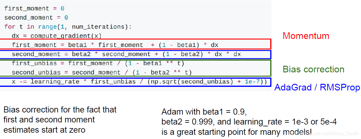
- It introduces a bias correction, which will be corrected when our initial momentum is relatively small.
1.5 Choice of learning rate
- In all our optimization algorithms, we need to formulate the initial learning rate, usually there are the following practices:
iterative period decay, exponential decay and fractional decay
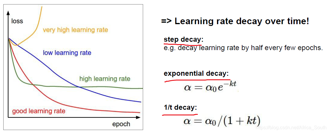
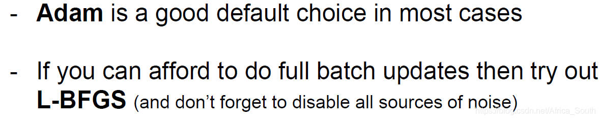
- Generally, learning rate attenuation is used when driving momentum SGD, but Adam can not be used. And instead of using step size attenuation as soon as you come up, you can debug other parameters first. You can try to decrease the learning rate when you observe the loss function is flat.
1.6 Second-Order Optimization (Second-Order Optimization)
- The previous optimization methods are all first-order optimization, that is, operations on the first-order partial derivatives.
-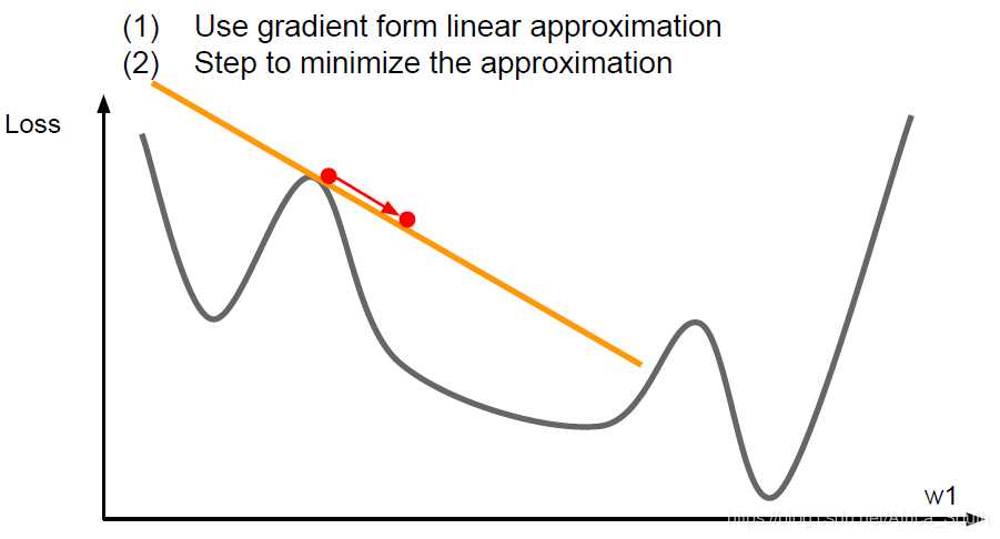
- It is equivalent to using the current point in the first-order Taylor expansion to approximate.
- So, we can also use the current point of the second-order Taylor expansion to approximate, while using the first-order and second order partial derivatives partial derivatives to be optimized:
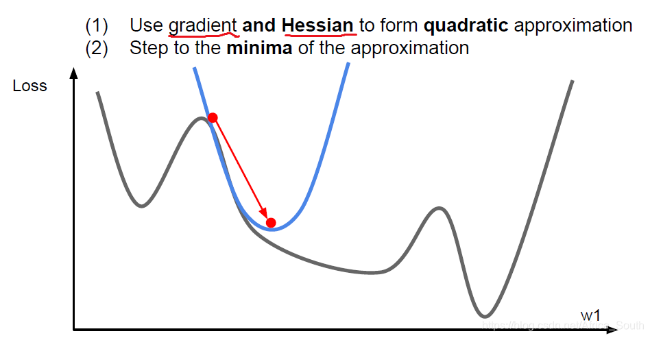
- One of the second-order optimization get our Newton step (Newton Step)
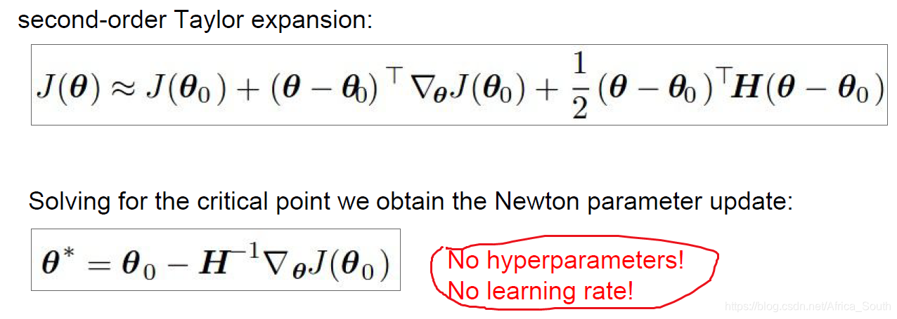
- Here we do not have the learning rate, because it was at that point the second-order Taylor expansion , and updates directly to the point at the minimum of the quadratic function. (But follow Newton descent method versions may add a learning rate).
- However, the inverse matrix is here seeking Heather in depth study impractical, so sometimes you can use a second-order approximation, that quasi-Newton method .
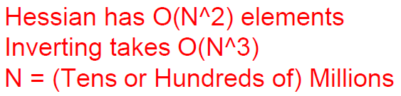
- Therefore, we also have a second-order optimizer- L-BFGS . But it may not be suitable for deep neural networks.
1.7 Model integration
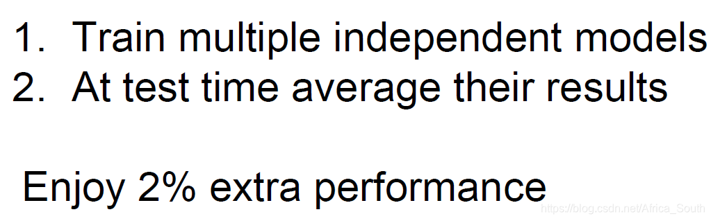
Before we talk about optimization algorithm, more often the relationship is how to get good enough performance in the training, but often we are more concerned about the performance of the model on the test set .
One solution is to use the model integration (Model Ensembles ), may be appropriate to slow over-fitting and super-parametric multiple models can be different
2. Regularization (Regularization)
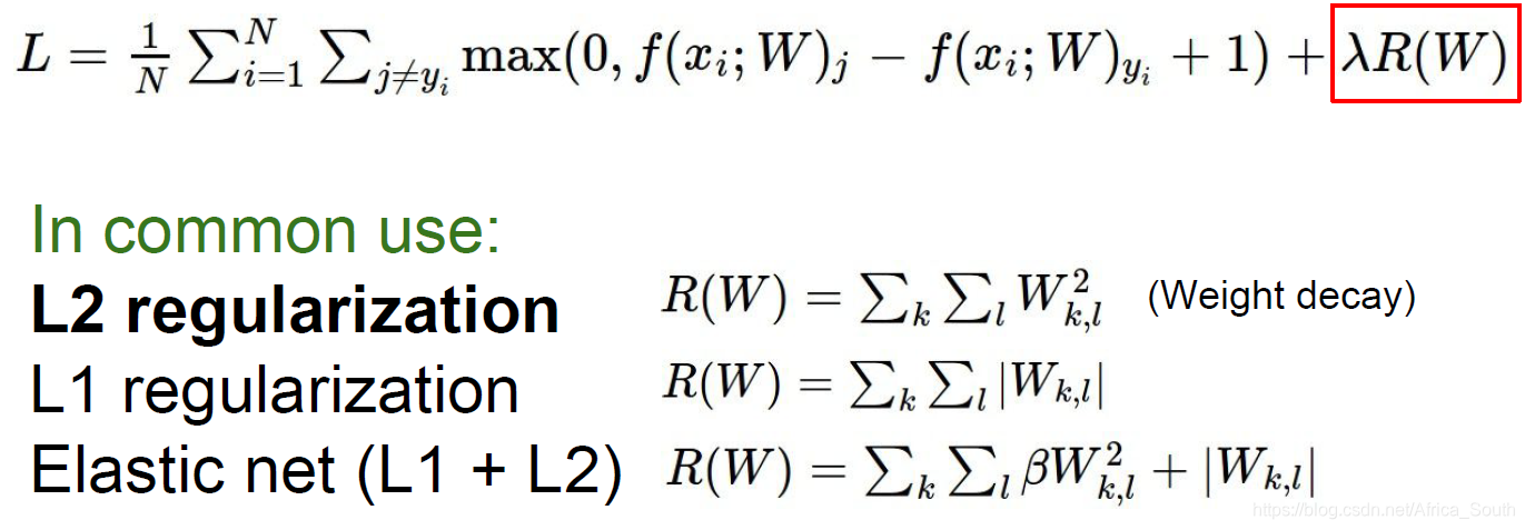
Another solution to improve the generalization ability of the model and reduce overfitting is regularization, which in a sense does not make the model too complicated.
2.1 Weight constraints
One way to regularize is to add norm constraints to the learning weights:
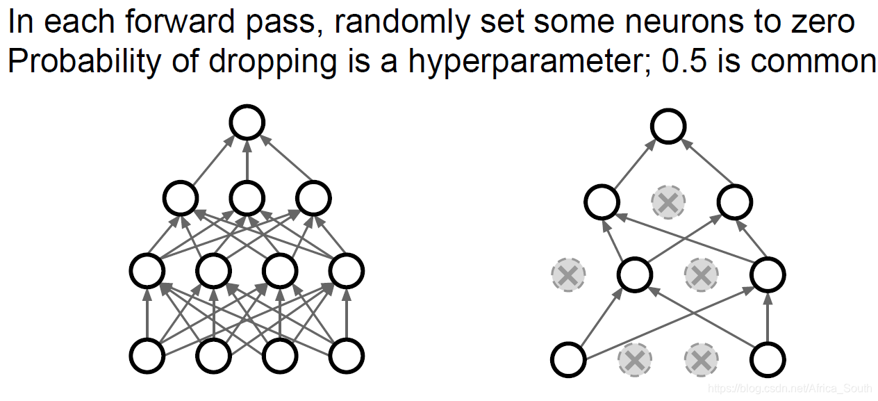
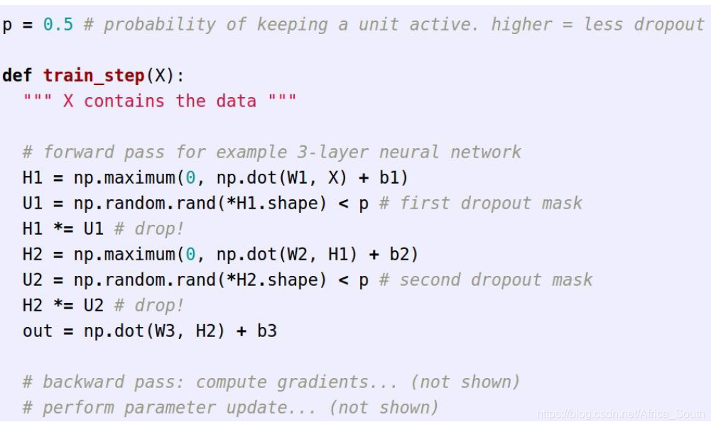
2.2 Random inactivation (Dropout)
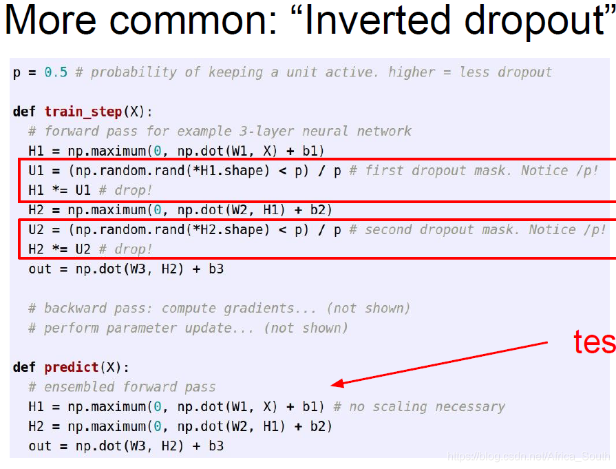
That is to say, when we are propagating in the forward direction, we randomly use the probability P to make the activation value of certain neurons in certain layers 0 , inactivating them.
For example, DP of a two-layer neural network:
explain
- The strong correlation between features can be avoided, so that the network can work normally only with partial features.
- Or as multiple sub-networks of integrated learning .
Test operation
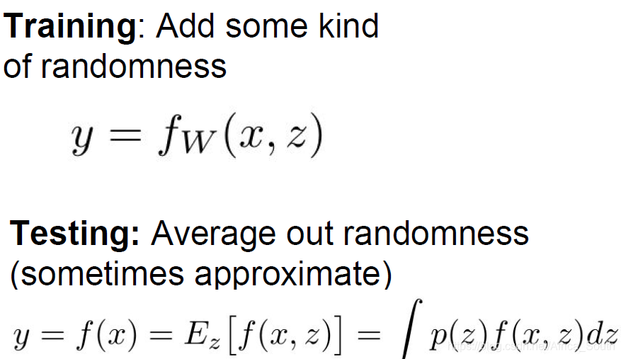
We randomly inactivated during the test, but what should we do during the test?
There must be no random inactivation, because this may cause the model to give different outputs for the same input.
Ideally, our input is the original input X and a mask Z, so we want to calculate the average value of this random Z:
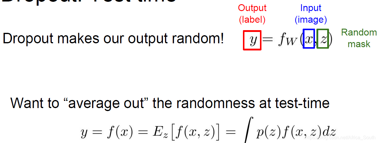
but this is quite difficult, so we can do a local approximation, assuming that we inactivation probability of 0.5:
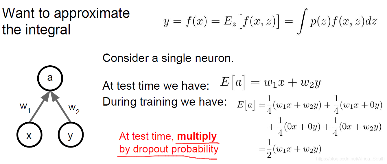
so, we just want our output value is multiplied by inactivation of probability can be.
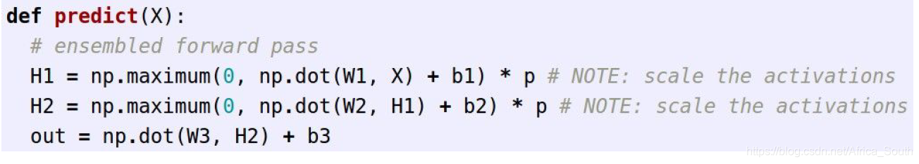
However, sometimes we don't want to introduce a matrix multiplication operation during the test, but put it in the training phase, because the training phase is usually performed on the GPU, so we can use "Inverted Dropout".
Promote
Similar to Dropout, we introduce some randomness during training to prevent it from overfitting the training data, and evenly offset its impact during testing.
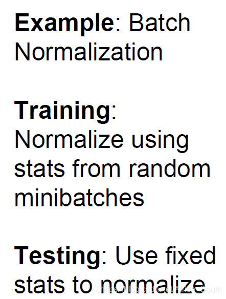
And we talked about before the bulk normalized BN is also in line with this strategy:
namely computing experience on a small lot in the training, but the emergence of a single batch data is random:
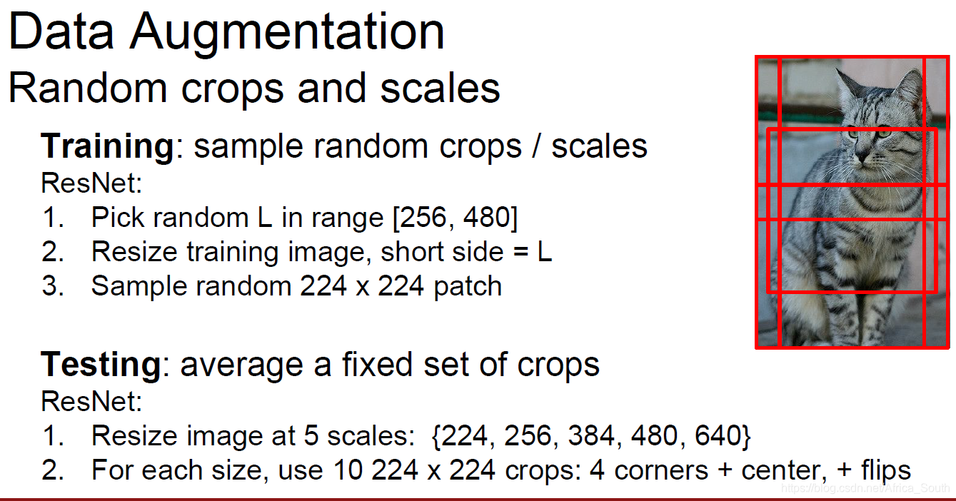
Of course, there is a similar strategy is carried out in the training of random data enhancement :
2.3 Local maximum pooling
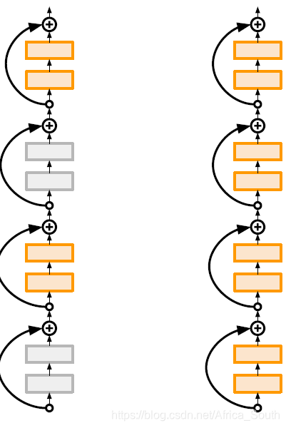
2.4 Random depth
That is, some network layers are randomly dropped during training, and all network layers are used during testing:
3. Transfer Learning
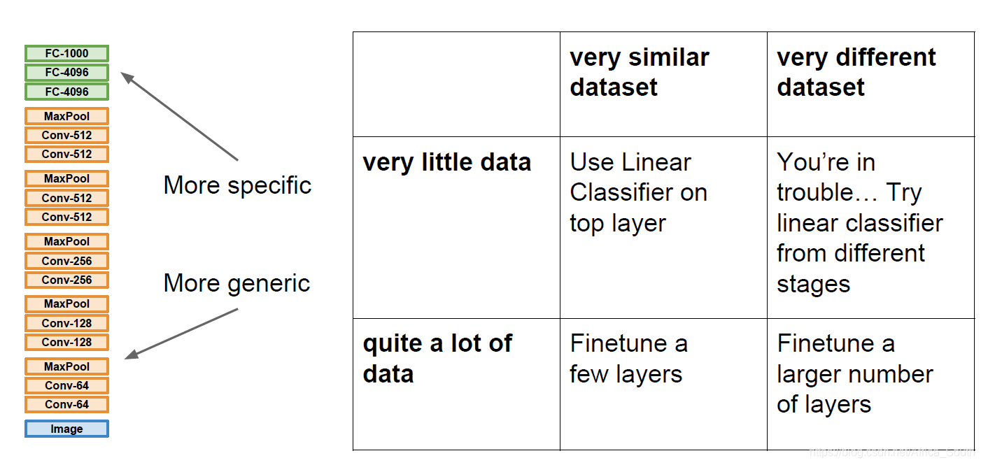
Transfer learning can reduce the degree of overfitting when training data is insufficient. It first trains a model on a large data set, and then applies its weight to a small data set, and makes appropriate adjustments (that is, freezing the weights of some layers unchanged, updating the weights of other layers).
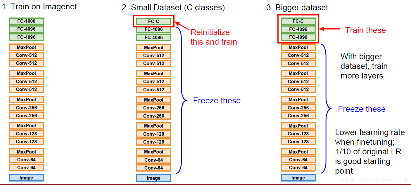
Generally, the characteristics of the CNN underlying It is a more general low-level and intermediate-level feature, so you can migrate and then fine-tune the head. For different situations, we adopt the following different strategies:
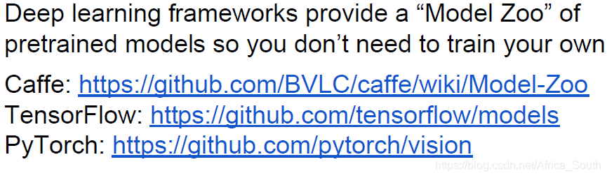
some existing neural network frameworks will also expose their own pre-training models:
to sum up