table of Contents
- Monte Carlo method overview
- Sampling method
- summary
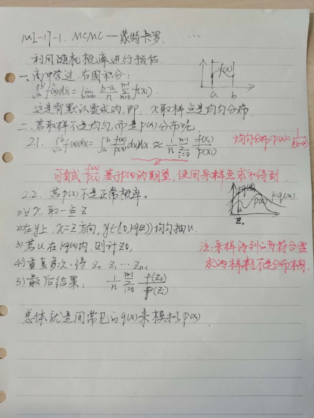
We can see from the name that MCMC consists of two MCs, namely Monte Carlo Simulation (MC) and Markov Chain (MC). This is because the restricted Boltzmann machine (RBM) needs to be applied, so first learn its principles. This article first explains the Monte Carlo method.
1. Overview of Monte Carlo Method
Monte Carlo ( Monte Carlo) was originally the name of a casino, and use it as the name probably because the Monte Carlo method is a stochastic simulation methods, procedures, much like throwing dice gambling games inside. The earliest Monte Carlo methods were designed to solve some summation or integration problems that are not very easy to solve, such as the area of a circle. Another example is points:

If f (x) is difficult to find its original function at this time, then this integral is very difficult to find. Of course, we can simulate the approximate value through the Monte Carlo method, assuming that our function f (x) is shown in the figure below
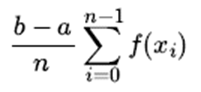
It can be known from learning knowledge in high school: assuming that the sampling data of x is uniformly distributed between [a, b], it can be solved by the differential and integral ideas, as shown in the following formula (when n is infinite, Value is the integral value):
The above assumption is evenly distributed, but in most cases, it is not evenly distributed between [a, b]. If we use the above method, the result of the simulation is likely to be far from the true value. How to solve this problem?
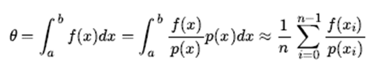
In general, we adopt a hypothetical approach: assuming the probability distribution function p (x) of x in [a, b], then the sum of our definite integrals can be carried out like this:
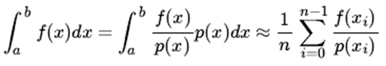
(Note that in the end, it is approximately equal to, approximately looking at the expected value of the former)
Assuming that the probability distribution is a uniform distribution, it is easy to convert it into the integral learned in high school:
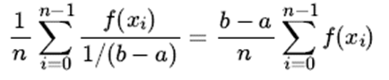
It can be seen that the two integral forms are the relationship between general and special cases.
Second, the sampling method
The key to the Monte Carlo method is the probability distribution obtained. If the probability distribution is found, we can use the probability distribution to sample the basis
The n sample sets of this probability distribution can be solved by introducing the Monte Carlo summation formula. But there is still a key problem to be solved, that is, how to obtain the n sample sets based on the sampling of this probability distribution.
2.1 Probability distribution sampling
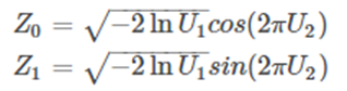
For the common uniformly distributed uniform (0, 1), it is very easy to sample samples. Generally, a linear congruential generator can easily generate pseudo-random number samples between (0, 1). For other common probability distributions, whether it is a discrete distribution or a continuous distribution, their samples can be obtained by transforming samples of uniform (0, 1). For example, two-dimensional normal distribution samples (Z1, Z2) can be obtained by uniform (0, 1) sample pairs (U1, U2) obtained by independent sampling through the following formula Box-Muller transformation :
In addition to the normal distribution, there are many other common continuous distributions (such as t distribution, F distribution, Beta distribution, Gamma distribution, etc.) can also be represented by a uniform 0-1 distribution, but many times our distribution is not common Distribution, which means that the probability distribution of the sample set cannot be obtained by these transformations.
However, in many cases, the probability distributions we encounter are not common distributions, which means that we cannot easily obtain sample sets of these very rare probability distributions. How to solve this problem?
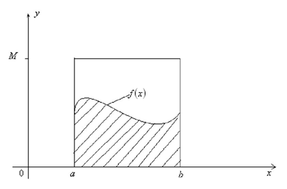
2.2 Accept - reject sampling
For the above problems, you can consider using accept-reject sampling to get samples of the distribution. Since p (x) is too complicated to directly sample in the program, I set a distribution q (x) that the program can sample, such as a Gaussian distribution, and then reject certain samples according to certain methods to achieve close to p (x) The purpose of distribution, where q (x) is called proposal distribution.
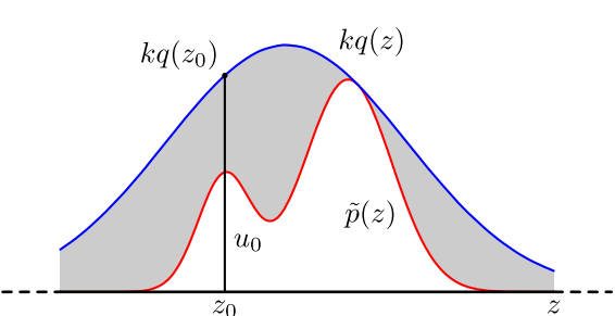
The specific operation is as follows, set a convenient sampling function q (x), and a constant k, so that p (x) is always below kq (x). (Refer to the picture above)
1) The x-axis direction: get z from the q (x) distribution sampling.
2) The y-axis direction: u is sampled from a uniform distribution (0, kq (z)).
3) If it happens to fall into the gray area: u> p (z), refuse, otherwise accept this sampling.
4) Repeat the above process to get n accepted samples, z0, z1, z2 ... z (n-1);
5) The final solution of Monte Carlo method is:
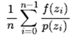
Throughout the process, we use a series of acceptance and rejection decisions to achieve the purpose of simulating the probability p (x) distribution with q (x).
3. Summary
Using accept-reject sampling, we can solve the purpose of obtaining the sampling set and summing it by Monte Carlo method when some probability distribution is not common. However, accept-reject sampling can only partially meet our needs. In many cases, it is still difficult for us to obtain a sample set of our probability distribution. such as:
1) For some two-dimensional distributions p (x, y), sometimes we can only get the sum of the conditional distributions p (x | y) and p (y | x), but it is difficult to get the two-dimensional distribution p (x, y) In general form, we cannot use accept-reject sampling to get its sample set.
2) For some high-dimensional complex uncommon distributions p (x1, x2, ..., xn), it is very difficult to find a suitable q (x) and k.
Mainly from: https://www.cnblogs.com/jiangxinyang/p/9358822.html
Annex I:
1. Box-Muller transformation principle link: https://blog.csdn.net/weixin_41793877/article/details/84700875
2. Explanation of the following inequalities:
In the last step of conversion, the integral on the left can be regarded as the expectation of f (x) / p (x) based on the probability distribution p (x), which can be solved by solving the expected average, that is, f (x) / p (x ) Based on the sampling points of the distribution p (x), and then find the tie value.
Appendix 2: Handwriting exercises