1. Learning content

1. Overview

Denoise the heart sound signal: (one week) the transmission gate
adopts spectral subtraction, Wiener filtering, LMS filter, NLMS filter, the noise reduction of the heart sound signal
uses residual noise, normalized root mean square MRMS, correlation coefficient, signal noise Indicators, comparing the noise reduction effects of LMS and NLMS
Recognize abnormal heart sounds: (one week ing)
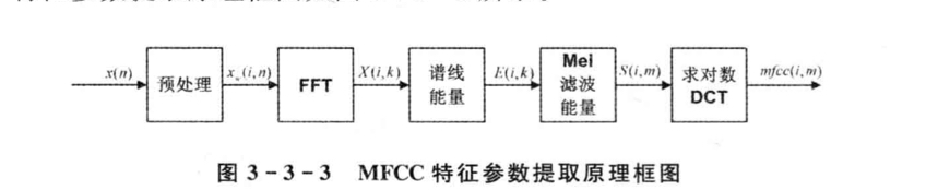
use MFCC to do feature extraction and
learn HMM hidden Markov model

2. Problems encountered

The evaluation of the noise reduction effect is very simple, and you should learn more comprehensive evaluation content
For LMS and NLMS, the error curve cannot be drawn (I tried a lot, I do n’t know where the problem is, I plan to ask my brother when the school starts)

3. Specific contents

Noise reduction

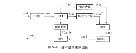
Spectral subtraction: Taking advantage of the feature that additive noise is not related to speech, assuming that the noise is statistically stable, the noise spectrum estimate measured without speech gaps is used to replace the frequency spectrum of noise during speech and subtracted from the noise-containing speech spectrum To obtain an estimate of the speech spectrum.
Input:
% signal Input signal sequence (column vector)
% NIS Leading non-speech frame number (scalar)
% fn Frame number (scalar)
% wlen Frame length (scalar)
% inc Frame shift (scalar)
% a Subtraction factor ( (Scalar)
% b gain compensation factor (scalar)
output:
% output_subspec spectral subtraction output waveform (column vector)

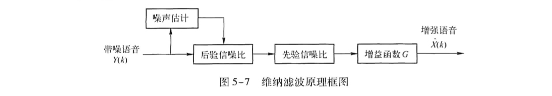
Wiener filtering:
Under the minimum mean square error criterion (MSE), the speech signal is estimated.
Input:
% x noisy speech signal
% IS Preamble without speech segment length
% T1 Threshold for judging whether there is speech
Output:
% Enhanced speech signal

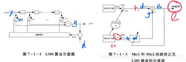
LMS filtering is
based on the minimum mean square value of the error between the expected response and the output signal of the filter . According to the input signal, the gradient vector is estimated in the iterative process and the weight coefficient is updated. (Gradient maximum descent method)
input:
% xn input signal sequence (column vector)
% dn desired response sequence (column vector)
% M filter order (scalar)
% mu convergence factor (step size) (scalar )
Output:
% W filter weight matrix (matrix)
% size is M x itr,
% e error sequence (itr x 1) (column vector)
% y actual output sequence (column vector)

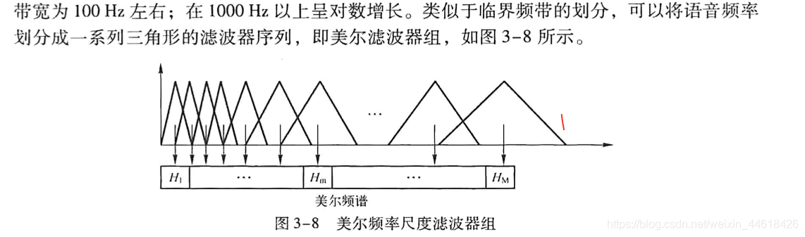
The
key of MFCC is to use Mel filter bank, which is more in line with the mechanism of auditory characteristics

HMM Hidden Markov
Establish HMM model (A, B, π) based on observations, predict state value
train: from "observation", find the HMM model (EM + forward-backward algorithm) most likely to produce "observation"
test: From the "observed value" and HMM model, get the best "state value" (Viterbi)

4. Reflection

When learning the principles of HMM, I just started to learn formula derivation directly. I did n’t clearly understand the way to solve the problem. After I went to the actual application and found that I did not understand it, I returned to continue to watch.

Therefore, when learning similar algorithms in the future, you should first understand clearly what
the problem is and what the solution is, and then pay attention to the detailed formula derivation.

Ask why, don't be too anxious.