I. Introduction
The main graph model learning is to learn the network structure, that is, to find the optimal network structure; and a network parameter estimation, that is known to the network structure, estimate the parameters of each conditional probability distribution. Here is mainly about network parameter estimation. Then the parameters can be divided into free estimate of hidden variables, and parameter estimation containing hidden variables. Hidden variable with respect to observable variables in terms of the variables that we can not directly observable; in the feature space can be understood in order to know the reasoning is characterized by not being directly visible, more advanced needs.
Second, the argument does not contain hidden variables estimates
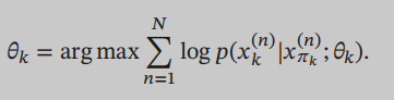
In a directed graph model, if all the variables are observable, but also know who is in the condition (parent), so long as the network parameters by maximum likelihood estimate can be estimated:
In order to reduce the parameter amount can be used to parameterize the model, if it is discrete can sigmoid belief networks, if continuous, you can use a Gaussian belief networks (answers on a blog doubts, the original Gaussian probability distribution also can be used, depends mainly on the variable x is discrete or continuous)
In a directed graph, the joint probability distribution of x will disassembled into the multiplicative group on the maximum of the potential energy function:
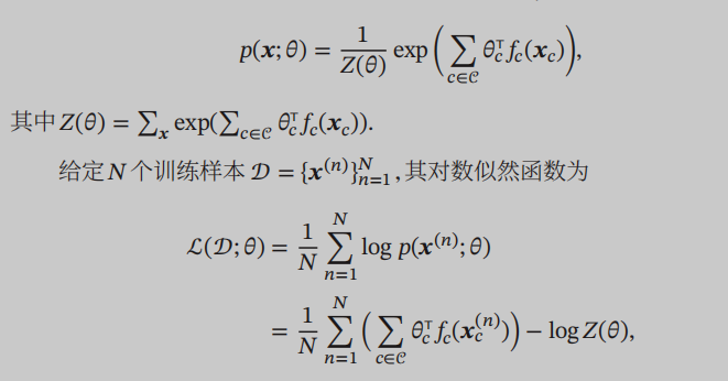
This derivative logarithm likelihood function theta similar parameters, can be found for the partition function Z derivative, the desired result is the distribution of the model:
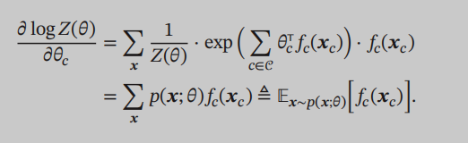
Distribution model here refers to the very beginning we define P (x), which is the subject of probability sample distribution, and our goal is to obtain the unknown parameters of the model.
Then we will find:

The first will inevitably reminiscent of the time just learning the indefinite integral, integration is the beginning of a rectangular area to be introduced. The first fact be called the empirical distribution, can also be written in the desired form:
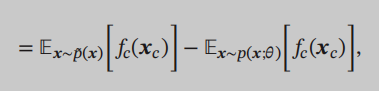
The former is empirical distribution, we get through the actual sample, which is the distribution model, we need requirements. We are beginning to make the derivative is the derivative equal to 0, calculated parameters, so undirected graph model, the derivation of this process is equivalent to our distribution through the sample to fit real.
Third, the estimation of parameters with Hidden Variables
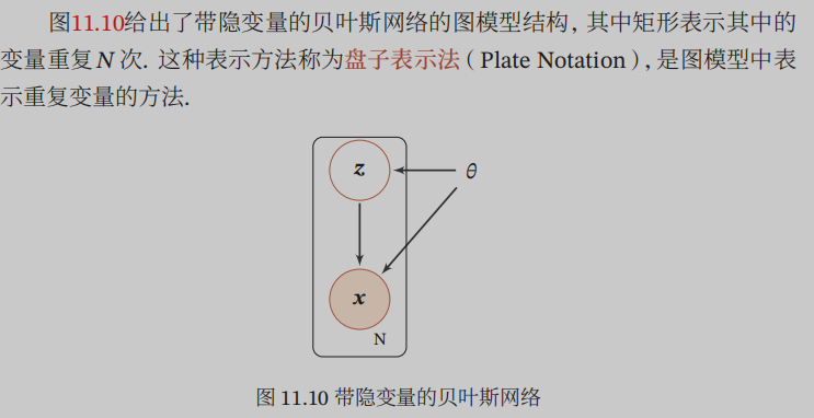
This model contains a hidden variable that is also contains observable variables, but always remember that we do not see the hidden variables are variables! Can we use the data sample only observable variables! No hidden variables! Because hidden variables can not see! Knowing this it is well understood next job!
In fact, the ultimate goal we require only p (x), x refers to the observable variables, latent variables are represented by z, first of all we could not find p (z), followed by seeking the p (z) there is no practical significance, we eat like a normal ultimate goal is to live, not to observe how rice is kind of digestion in the stomach, although these researchers studied only enriched our medical treasure, but they study the researchers of this ultimate goal It is scientific research, but also to eat people alive!
How that beg p (x) it, we now know that there are two random variables in the model, observable and hidden, then they will relate to each other, but we can only see random variables observable, invisible hidden, but hidden variables are random variables, they also affect the probability of our observable variables, although we do not need to figure out specifically how the distribution of hidden variables, but we have to take into consideration the hidden variables observable variables probability distribution Effects of.
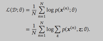
Defined sample x marginal likelihood function is: $ p (x; \ theta) = \ sum_ {z} ^ {} p (x, z; \ theta) $
This formula tells us that if you want to know the probability distribution of the observable variable x, as long as the joint probability of observable variables x and z, and then the implicit variable z summing enough, in fact, seek marginal probability of x, because here random That non-variable x z, x is the marginal probability of z joint probability summation. See here before when I feel good nonsense ah, if I know the joint probability distribution, it must be able to seek out well, but the key is hidden variables can not see, can not seek first the joint probability distribution and then summing Well, according to this ideas, if still using the previous graph model without hidden variables mentioned in the likelihood, then, to maximize the likelihood estimation:
Even this likelihood function direct derivation, we also found that the log derivation, the joint probability distribution will go to the denominator, we can not eliminate that we have not calculated the joint probability distribution. This sum can not be calculated directly, it will lead to a problem called the inference problem, in fact, concluded that the main problem is to calculate the conditional probability distribution $ p (z \ mid x; \ theta) $, why this calculation, because the joint probability distribution $ p (z, x; \ theta) = p (z \ mid x; \ theta) p (x; \ theta) $, why the joint probability distribution can not be considered mainly involving sums of z, we follow the joint probability distribution after decomposition conditional probability formula, wherein the term containing z is the conditional probability distribution $ p (z \ mid x; \ theta) $, if we calculate this value, the likelihood function is also no problem. Inferred deduced exact and approximate inference, then there arise out of a lot of knowledge, on the other blog to write.
Now take a step back likelihood function is less than the sum of that step Z, the likelihood function is mainly to calculate the $ log p (x; \ theta) $