Python房价分析和可视化＜anjuke二手房＞

Python房价分析和可视化＜anjuke二手房＞

本文是Python数据分析实战的房价分析系列，本文分析二线城市贵阳的二手房。
数据获取
本文的数据来源于2022年7月anjuke的二手房数据。对数据获取不感兴趣可以跳过此部分看分析和可视化。
anjuke二手房数据和新房数据一样，不需要抓包，直接拼接url即可。步骤如下：
1.访问目标页面
进入网站首页，点击选择城市和二手房进入<二手房信息页面>，筛选条件（位置、价格等）都保持默认，这样可以查出全部二手房信息。

2.分析url变化
拖动滚动条到翻页的地方，点击几次<上一页>、<下一页>翻页，观察浏览器上方搜索框里url的变化。可以看到每次翻页url只变化一个数字，对应当前的页数。
所以只要不断改变url中的页数，就可以获取所有的数据。
3.二手房总页数分析
二手房不像新房，新房的楼盘数有限，二手房数量很多，已经超过了网站的最大显示数量，anjuke最多展示50页二手房数据，所以我们要获取的数据总页数为50。anjuke二手房前面有部分页面的信息为每页87条，后面的页面是每页60条，所以一共可以获取到3000多条房源信息。
4.循环拼接url获取所有数据
在url中从1开始拼接页数，直到第50页，依次获取所有页面的信息。
参考代码：

import random
import time

for p in range(1, 51):
     time.sleep(random.randint(10, 30))
     second_house_url = 'https://gy.anjuke.com/sale/p{}'.format(p)
     try:
         res = requests.get(second_house_url, headers=headers)  # headers需要自己准备
         print('获取第{}页数据成功'.format(p))
     except Exception as e:
         print('获取第{}页数据失败，报错：{}'.format(p, e))

5.用XPath提取数据
anjuke二手房信息在返回结果的HTML文件中，需要使用XPath语法提取。
参考代码：

from lxml import etree

result = res.text
html = etree.HTML(result)
infos = html.xpath("//section[@class='list-left']/section[2]/div")

XPath快速入门参考：快速入门XPath语法，轻松解析爬虫时的HTML内容
用XPath获取当前页的所有二手房信息保存在infos中，infos是一个Element对象的列表，每一个Element对象里的信息是一条二手房信息，可以继续用XPath从中提取具体的信息。
6.将数据保存到excel中
使用pandas将解析的数据转换成DataFrame，然后保存到excel中。最终获取到的数据共3135条。

获取数据时可能会遇到验证码，anjuke有两种验证码，一种是拖动滑块，一种是点击指定图形下的字符。遇到验证码时，手动在浏览器页面上点击通过验证再跑代码就行了。
除了会遇到验证码，如果访问比较频繁，还可能会被封ip，初次被封只会封两个小时左右，假如连续被封可能会被永久封。所以本文的代码中每个页面的间隔时间设置得比较长，并且每次访问更换headers中的user_agent。有条件的话也可以设置ip池，使用代理。

数据清洗
二手房的信息比较完整，只需要简单的清洗。
1.删除重复值

# coding=utf-8
import pandas as pd
import numpy as np

df = pd.read_excel('anjuke_second_house.xlsx', index_col=False)
print(df.shape)
# 删除重复值
df.drop_duplicates('标题', inplace=True)
print(df.shape)

(3135, 12)
(3022, 12)

删除重复值后，剩下的二手房信息为3022条。
2.填充空值

# 空值填充
print(np.any(df.isnull()))
df.fillna('未知', inplace=True)
print(np.any(df.isnull()))

True
False

数据准备好后，本文开始对获取的3022条二手房信息进行分析。
二手房所属楼盘Top30

from pyecharts.charts import Bar
from pyecharts import options as opts

# 二手房数量Top30的楼盘
second_build_name = df['楼盘'].value_counts()[0:30]
bar = Bar(init_opts=opts.InitOpts(width='1000px', height='400px', bg_color='white'))
bar.add_xaxis(
    second_build_name.index.to_list()
).add_yaxis(
    '', second_build_name.to_list(), category_gap='30%'
).set_global_opts(
    title_opts=opts.TitleOpts(title='二手房数量前30的楼盘', pos_left='400', pos_top='30',
        title_textstyle_opts=opts.TextStyleOpts(color='black', font_size=16)),
    xaxis_opts=opts.AxisOpts(axislabel_opts=opts.LabelOpts(font_size=10, distance=0, rotate=30, color='#4863C4'))
).set_colors('#4863C4').render('second_build_name_top30.html')

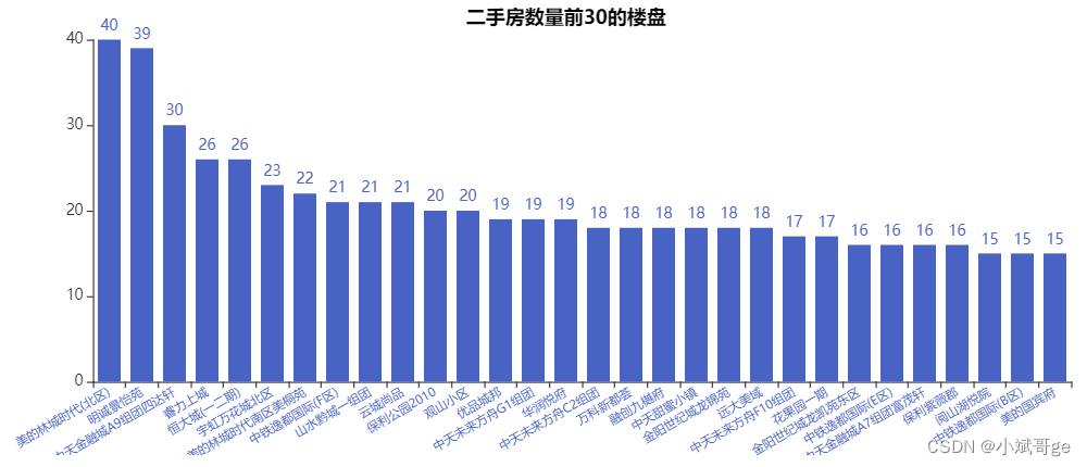在二手房的所属楼盘中，“中天”开头的楼盘最多，在购买这个房开的新房时也需要谨慎，那么多人要转卖说不定有什么坑，如物业不好、房开降标等。
二手房的单价分布

from pyecharts.charts import Pie
from pyecharts import options as opts

# 获取各个价格区间的二手房数量
second_price_unit = df['单价']
sections = [0, 5000, 6000, 7000, 8000, 9000, 10000, 12000, 15000, 20000, 100000]
group_names = ['less-5k', '5k-6k', '6k-7k', '7k-8k', '8k-9k', '9k-1w', '1w-1w2', '1w2-1w5', '1w5-2w', 'surpass-2w']
cuts = pd.cut(np.array(second_price_unit), sections, labels=group_names)
second_counts = pd.value_counts(cuts, sort=False)
pie = Pie(init_opts=opts.InitOpts(width='800px', height='600px', bg_color='white'))
pie.add(
    '', [list(z) for z in zip([gen for gen in second_counts.index], second_counts)],
    radius=['20%', '70%'], rosetype="radius", center=['60%', '50%']
).set_series_opts(
    label_opts=opts.LabelOpts(formatter="{b}: {c}"),
).set_global_opts(
    title_opts=opts.TitleOpts(title='二手房单价分布情况', pos_left='400', pos_top='30',
        title_textstyle_opts=opts.TextStyleOpts(color='black', font_size=16)),
    legend_opts=opts.LegendOpts(is_show=False)
).render('second_price_counts.html')

从单价看，大部分二手房的单价在6k-1w之间，最多的单价是7k-8k。
二手房的总价分布

from pyecharts.charts import Pie
from pyecharts import options as opts

# 获取二手房总价各区间的数量
second_price_total = df['总价']
sections = [0, 50, 60, 70, 80, 90, 100, 120, 150, 200, 250, 10000]
group_names = ['less-50w', '50w-60w', '60w-70w', '70w-80w', '80w-90w', '90w-100w', '100w-120w', '120w-150w', '150w-200w', '200w-250w', 'surpass-250w']
cuts = pd.cut(np.array(second_price_total), sections, labels=group_names)
second_counts = pd.value_counts(cuts)
pie = Pie(init_opts=opts.InitOpts(width='800px', height='600px', bg_color='white'))
pie.add(
    '', [list(z) for z in zip([gen for gen in second_counts.index], second_counts)],
    radius=['20%', '70%'], rosetype="radius", center=['50%', '50%']
).set_series_opts(
    label_opts=opts.LabelOpts(formatter="{b}: {c}"),
).set_global_opts(
    title_opts=opts.TitleOpts(title='二手房总价分布情况', pos_left='330', pos_top='20',
        title_textstyle_opts=opts.TextStyleOpts(color='black', font_size=16)),
    legend_opts=opts.LegendOpts(is_show=False)
).set_colors(
    ['rgb(0,{g},{b})'.format(g=100+10*x, b=200-15*x) for x in range(12)]
).render('second_total_price_counts.html')

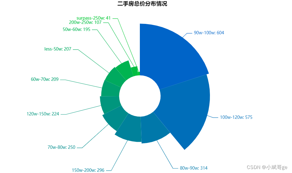差不多有一半二手房的总价在80w-120w之间，其中90w-120w的数量最多。
二手房的区域分布

from pyecharts.charts import Map
from pyecharts import options as opts

# 获取二手房的位置信息
second_house_location = df['地址'].copy()
second_house_location = second_house_location.apply(lambda x: x.split('-')[0]).value_counts()
data_pair = [['观山湖区', int(second_house_location['观山湖'])], ['云岩区', int(second_house_location['云岩'])],
             ['南明区', int(second_house_location['南明'])], ['白云区', int(second_house_location['白云'])],
             ['清镇市', int(second_house_location['清镇'])], ['乌当区', int(second_house_location['乌当'])],
             ['花溪区', int(second_house_location['花溪']) + int(second_house_location['小河经开区'])]]
map = Map(init_opts=opts.InitOpts(bg_color='black', width='1000px', height='700px'))
map.add(
    '', data_pair=data_pair, maptype="贵阳"
).set_global_opts(
    title_opts=opts.TitleOpts(title='贵阳各区二手房分布', pos_left='400', pos_top='50',
                              title_textstyle_opts=opts.TextStyleOpts(color='white', font_size=16)),
    visualmap_opts=opts.VisualMapOpts(max_=1200, is_piecewise=True, pos_left='100', pos_bottom='100',
                                      textstyle_opts=opts.TextStyleOpts(color='white', font_size=16))
).render("second_house_location.html")

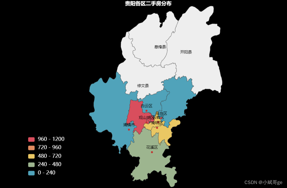从区域看，观山湖区的二手房最多，超过了1000套，占比约1/3。所属贵阳的三个县在anjuke上没有二手房信息。
观山湖区二手房总价分布

from pyecharts.charts import Pie
from pyecharts import options as opts

# 获取观山湖二手房总价各区间的数量
second_house_location = df['地址'].copy()
second_house_location = second_house_location.apply(lambda x: x.split('-')[0])
second_house_core = second_house_location[second_house_location == '观山湖']
second_price_total_core = df.loc[second_house_core.index, '总价']
sections = [0, 50, 80, 90, 100, 120, 150, 200, 250, 10000]
group_names = ['less-50w', '50w-80w', '80w-90w', '90w-100w', '100w-120w', '120w-150w', '150w-200w', '200w-250w', 'surpass-250w']
cuts = pd.cut(np.array(second_price_total_core), sections, labels=group_names)
second_counts = pd.value_counts(cuts)
pie = Pie(init_opts=opts.InitOpts(width='800px', height='600px', bg_color='white'))
pie.add(
    '', [list(z) for z in zip([gen for gen in second_counts.index], second_counts)],
    radius=['20%', '60%'], rosetype="radius", center=['50%', '50%']
).set_series_opts(
    label_opts=opts.LabelOpts(formatter="{b}: {c}"),
).set_global_opts(
    title_opts=opts.TitleOpts(title='观山湖区二手房总价分布情况', pos_left='300', pos_top='20',
        title_textstyle_opts=opts.TextStyleOpts(color='black', font_size=16)),
    legend_opts=opts.LegendOpts(is_show=False)
).set_colors(
    ['rgb({r},0,{b})'.format(r=150-15*x, b=100+15*x) for x in range(11)]
).render('second_price_total_core.html')

观山湖区作为贵阳二手房最多的区，有近3/4二手房的总价在90w-200w之间，其中有近3成总价在100w-120w之间。整体来看，观山湖区的总价属于贵阳市的总价中偏高的部分。
二手房户型分布

from pyecharts.charts import Bar
from pyecharts import options as opts

# 获取二手房的户型分布
second_house_type = df['户型'].value_counts()
second_house_type_parse = second_house_type.loc[second_house_type >= 10]
second_house_type_parse['others'] = second_house_type.loc[second_house_type < 10].sum()
bar = Bar(init_opts=opts.InitOpts(width='1000px', height='400px', bg_color='white'))
bar.add_xaxis(
    second_house_type_parse.index.to_list()
).add_yaxis(
    '', second_house_type_parse.to_list(), category_gap='30%'
).set_global_opts(
    title_opts=opts.TitleOpts(title='二手房户型数量分布', pos_left='420', pos_top='30',
        title_textstyle_opts=opts.TextStyleOpts(color='black', font_size=16)),
    xaxis_opts=opts.AxisOpts(axislabel_opts=opts.LabelOpts(font_size=12, distance=0, rotate=20, color='#FF9366')),
    yaxis_opts=opts.AxisOpts(max_=1400)
).set_colors('#FF9366').render('second_house_type.html')

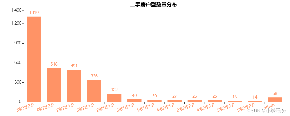大部分二手房的户型都是3室2厅2卫，这种户型不仅是二手房的主力户型，其实也是新房的主力户型，符合大部分购房者的需求。
二手房面积分布

from pyecharts.charts import Pie
from pyecharts import options as opts

# 获取二手房的面积分布情况
second_area = df['面积']
sections = [0, 50, 80, 90, 100, 110, 120, 130, 140, 150, 200, 10000]
group_names = ['0-50㎡', '50-80㎡', '80-90㎡', '90-100㎡', '100-110㎡', '110-120㎡', '120-130㎡', '130-140㎡', '140-150㎡', '150-200㎡', '200㎡以上']
cuts = pd.cut(np.array(second_area), sections, labels=group_names)
second_area_counts = pd.value_counts(cuts, ascending=True)
pie = Pie(init_opts=opts.InitOpts(width='800px', height='600px', bg_color='white'))
pie.add(
    '', [list(z) for z in zip([gen for gen in second_area_counts.index], second_area_counts)],
    radius=['20%', '70%'], rosetype="radius", center=['50%', '50%']
).set_series_opts(
    label_opts=opts.LabelOpts(formatter="{b}: {c}"),
).set_global_opts(
    title_opts=opts.TitleOpts(title='二手房面积分布情况', pos_left='330', pos_top='20',
        title_textstyle_opts=opts.TextStyleOpts(color='black', font_size=16)),
    legend_opts=opts.LegendOpts(is_show=False)
).set_colors(
    ['rgb({r},0,{b})'.format(r=20*x, b=250-15*x) for x in range(12)]
).render('second_area_counts.html')

超过一半的二手房面积在110平到140平之间，在120平到140平之间的二手房最多。
二手房朝向分布

from pyecharts.charts import Pie
from pyecharts import options as opts

# 统计二手房的朝向
second_house_toward = df['朝向'].value_counts()
pie = Pie(init_opts=opts.InitOpts(width='800px', height='600px', bg_color='white'))
pie.add(
    '', [list(z) for z in zip([gen for gen in second_house_toward.index], second_house_toward)],
    radius=['40%', '60%'], center=['50%', '50%']
).set_series_opts(
    label_opts=opts.LabelOpts(formatter="{b}: {c}"),
).set_global_opts(
    title_opts=opts.TitleOpts(title='二手房朝向分布情况', pos_left='330', pos_top='20',
        title_textstyle_opts=opts.TextStyleOpts(color='black', font_size=16)),
    legend_opts=opts.LegendOpts(is_show=False)
).render('second_house_toward.html')

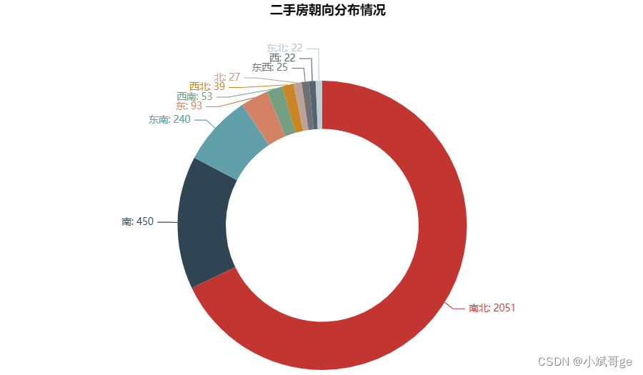南北朝向的二手房接近8成，如果加上东南、西南朝向，就接近了9成。南北朝向主要是为了减少阳光直射的时长，从这个分布来看，贵阳的二手房大部分都是南北朝向，因此朝向不能作为二手房的卖点。
二手房的修建年份

from pyecharts.charts import Bar
from pyecharts import options as opts

# 获取二手房的修建年份
second_house_build_year = df['年限'].copy().value_counts()
unknown = second_house_build_year['未知']
second_house_build_year.drop('未知', inplace=True)
second_house_build_year.index = [y[0:4] for y in second_house_build_year.index.to_list()]
second_house_build_year = second_house_build_year.sort_index(ascending=False)
second_house_build_year['未知'] = unknown
bar = Bar(init_opts=opts.InitOpts(width='1000px', height='400px', bg_color='white'))
bar.add_xaxis([i for i in second_house_build_year.index]).add_yaxis(
    '', second_house_build_year.to_list(), category_gap='20%'
).set_series_opts(
    label_opts=opts.LabelOpts(font_size=12)
).set_global_opts(
    title_opts=opts.TitleOpts(title='二手房修建年份分布', pos_left='420', pos_top='20',
        title_textstyle_opts=opts.TextStyleOpts(color='black', font_size=16)),
    yaxis_opts=opts.AxisOpts(max_=400),
    xaxis_opts=opts.AxisOpts(axislabel_opts=opts.LabelOpts(font_size=10, rotate=30, interval=0, color='#4863C4'))
).set_colors(['#4863C4']).render('second_house_build_year.html')

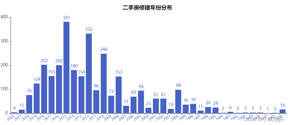二手房的修建年份大部分在3年-15年间，最多的三个年份是2015年、2012年和2010年。
二手房信息的标题风格

import jieba
from wordcloud import WordCloud
from PIL import Image

second_house_title = df['标题']
title_content = ','.join([str(til.replace(' ', '')) for til in second_house_title.to_list()])
cut_text = jieba.cut(title_content)
result = ' '.join(cut_text)
shape = np.array(Image.open("ciyun001.png"))
exclude = {
    
    '满二'}
wc = WordCloud(font_path="simhei.ttf", max_font_size=70, background_color='white', colormap='winter',
               stopwords=exclude, prefer_horizontal=1, mask=shape, relative_scaling=0.1)
wc.generate(result)
wc.to_file("second_house_title.png")

在海量的二手房信息中，起一个好标题无疑可以吸引更多潜在买家点击，还有可能提高成交几率。在这3000多条二手房信息的标题中，高频出现的词主要有精装修、拎包入住、地铁口、南北通透(当然这点前面已经证明不算卖点)、随时看房、急售、几室几厅、多少万等。
总结
本文获取了anjuke上贵阳市的二手房数据，对数据进行各个维度的分析，并用Python进行可视化。
文中用到的Python库和工具以后会专门写文章详细介绍，对代码有疑问可以关注和联系我一起交流讨论，欢迎点赞、评论和收藏。