Python中的图像处理（第十四章）Python图像分割（2）

前言

随着人工智能研究的不断兴起，Python的应用也在不断上升，由于Python语言的简洁性、易读性以及可扩展性，特别是在开源工具和深度学习方向中各种神经网络的应用，使得Python已经成为最受欢迎的程序设计语言之一。由于完全开源，加上简单易学、易读、易维护、以及其可移植性、解释性、可扩展性、可扩充性、可嵌入性：丰富的库等等，自己在学习与工作中也时常接触到Python，这个系列文章的话主要就是介绍一些在Python中常用一些例程进行仿真演示！

本系列文章主要参考杨秀章老师分享的代码资源，杨老师博客主页是Eastmount，杨老师兴趣广泛，不愧是令人膜拜的大佬，他过成了我理想中的样子，希望以后有机会可以向他请教学习交流。

因为自己是做图像语音出身的，所以结合《Python中的图像处理》，学习一下Python相关，OpenCV已经在Python上进行了多个版本的维护，所以相比VS，Python的环境配置相对简单，缺什么库直接安装即可。本系列文章例程都是基于Python3.8的环境下进行，所以大家在进行借鉴的时候建议最好在3.8.0版本以上进行仿真。本文继续来对本书第十四章的5个例程进行介绍。

一. Python准备

如何确定自己安装好了python

win+R输入cmd进入命令行程序

点击“确定”

输入：python，回车

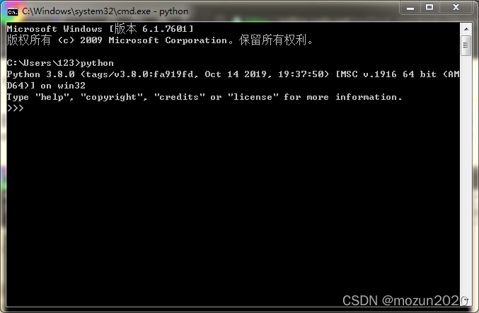
看到Python相关的版本信息，说明Python安装成功。

二. Python仿真

（1）新建一个chapter14_06.py文件，输入以下代码，图片也放在与.py文件同级文件夹下

# coding: utf-8
# 2021-05-17 Eastmount CSDN
import cv2
import numpy as np
import matplotlib.pyplot as plt

#读取原始图像
img = cv2.imread('scenery.png') 
print(img.shape)

#图像二维像素转换为一维
data = img.reshape((-1,3))
data = np.float32(data)

#定义中心 (type,max_iter,epsilon)
criteria = (cv2.TERM_CRITERIA_EPS +
            cv2.TERM_CRITERIA_MAX_ITER, 10, 1.0)

#设置标签
flags = cv2.KMEANS_RANDOM_CENTERS

#K-Means聚类 聚集成2类
compactness, labels2, centers2 = cv2.kmeans(data, 2, None, criteria, 10, flags)

#K-Means聚类 聚集成4类
compactness, labels4, centers4 = cv2.kmeans(data, 4, None, criteria, 10, flags)

#K-Means聚类 聚集成8类
compactness, labels8, centers8 = cv2.kmeans(data, 8, None, criteria, 10, flags)

#K-Means聚类 聚集成16类
compactness, labels16, centers16 = cv2.kmeans(data, 16, None, criteria, 10, flags)

#K-Means聚类 聚集成64类
compactness, labels64, centers64 = cv2.kmeans(data, 64, None, criteria, 10, flags)

#图像转换回uint8二维类型
centers2 = np.uint8(centers2)
res = centers2[labels2.flatten()]
dst2 = res.reshape((img.shape))

centers4 = np.uint8(centers4)
res = centers4[labels4.flatten()]
dst4 = res.reshape((img.shape))

centers8 = np.uint8(centers8)
res = centers8[labels8.flatten()]
dst8 = res.reshape((img.shape))

centers16 = np.uint8(centers16)
res = centers16[labels16.flatten()]
dst16 = res.reshape((img.shape))

centers64 = np.uint8(centers64)
res = centers64[labels64.flatten()]
dst64 = res.reshape((img.shape))

#图像转换为RGB显示
img = cv2.cvtColor(img, cv2.COLOR_BGR2RGB)
dst2 = cv2.cvtColor(dst2, cv2.COLOR_BGR2RGB)
dst4 = cv2.cvtColor(dst4, cv2.COLOR_BGR2RGB)
dst8 = cv2.cvtColor(dst8, cv2.COLOR_BGR2RGB)
dst16 = cv2.cvtColor(dst16, cv2.COLOR_BGR2RGB)
dst64 = cv2.cvtColor(dst64, cv2.COLOR_BGR2RGB)

#用来正常显示中文标签
plt.rcParams['font.sans-serif']=['SimHei']

#显示图像
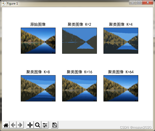
titles = [u'原始图像', u'聚类图像 K=2', u'聚类图像 K=4',
          u'聚类图像 K=8', u'聚类图像 K=16',  u'聚类图像 K=64']  
images = [img, dst2, dst4, dst8, dst16, dst64]  
for i in range(6):  
   plt.subplot(2,3,i+1), plt.imshow(images[i], 'gray'), 
   plt.title(titles[i])  
   plt.xticks([]),plt.yticks([])  
plt.show()

保存.py文件
输入eixt()退出python，输入命令行进入工程文件目录

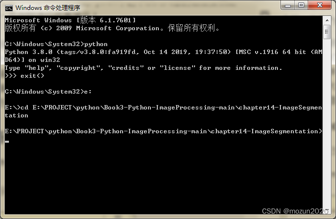
输入以下命令，跑起工程

python chapter14_06.py

没有报错，直接打印数据，弹出图片，运行成功！

（2）新建一个chapter14_07.py文件，输入以下代码，图片也放在与.py文件同级文件夹下

# coding: utf-8
# 2021-05-17 Eastmount CSDN
import cv2
import numpy as np
import matplotlib.pyplot as plt

#读取原始图像灰度颜色
img = cv2.imread('scenery.png') 

spatialRad = 100   #空间窗口大小
colorRad = 100     #色彩窗口大小
maxPyrLevel = 2    #金字塔层数

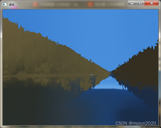
#图像均值漂移分割
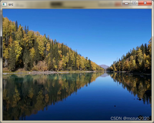
dst = cv2.pyrMeanShiftFiltering( img, spatialRad, colorRad, maxPyrLevel)

#显示图像
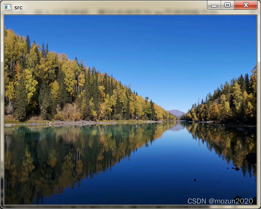
cv2.imshow('src', img)
cv2.imshow('dst', dst)
cv2.waitKey()
cv2.destroyAllWindows()

保存.py文件输入以下命令，跑起工程

python chapter14_07.py

没有报错，直接弹出图片，运行成功！


（3）新建一个chapter14_08.py文件，输入以下代码，图片也放在与.py文件同级文件夹下

# coding: utf-8
# 2021-05-17 Eastmount CSDN
import cv2
import numpy as np
import matplotlib.pyplot as plt

#读取原始图像灰度颜色
img = cv2.imread('scenery.png') 

#获取图像行和列
rows, cols = img.shape[:2]

#mask必须行和列都加2且必须为uint8单通道阵列
mask = np.zeros([rows+2, cols+2], np.uint8) 

spatialRad = 100 #空间窗口大小
colorRad = 100   #色彩窗口大小
maxPyrLevel = 2  #金字塔层数

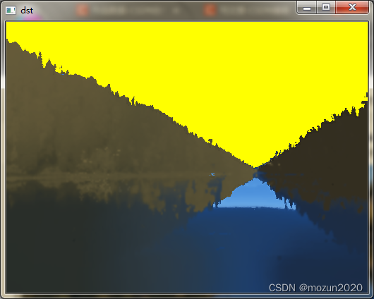
#图像均值漂移分割
dst = cv2.pyrMeanShiftFiltering( img, spatialRad, colorRad, maxPyrLevel)

#图像漫水填充处理
cv2.floodFill(dst, mask, (30, 30), (0, 255, 255),
              (100, 100, 100), (50, 50, 50),
              cv2.FLOODFILL_FIXED_RANGE)

#显示图像
cv2.imshow('src', img)
cv2.imshow('dst', dst)
cv2.waitKey()
cv2.destroyAllWindows()

保存.py文件输入以下命令，跑起工程

python chapter14_08.py

没有报错，直接弹出图片，运行成功！

（4）新建一个chapter14_09.py文件，输入以下代码，图片也放在与.py文件同级文件夹下

# coding: utf-8
# 2021-05-17 Eastmount CSDN
import numpy as np
import cv2
from matplotlib import pyplot as plt

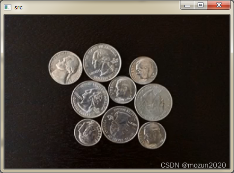
#读取原始图像
img = cv2.imread('test01.png')

#图像灰度化处理
gray = cv2.cvtColor(img,cv2.COLOR_BGR2GRAY)

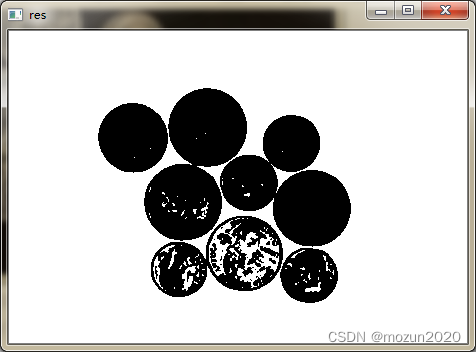
#图像阈值化处理
ret, thresh = cv2.threshold(gray, 0, 255, 
cv2.THRESH_BINARY_INV+cv2.THRESH_OTSU)

#显示图像
cv2.imshow('src', img)
cv2.imshow('res', thresh)
cv2.waitKey()
cv2.destroyAllWindows()

保存.py文件输入以下命令，跑起工程

python chapter14_09.py

没有报错，直接弹出图片，运行成功！

（5）新建一个chapter14_10.py文件，输入以下代码，图片也放在与.py文件同级文件夹下

# coding: utf-8
# 2021-05-17 Eastmount CSDN
import numpy as np
import cv2
from matplotlib import pyplot as plt

#读取原始图像
img = cv2.imread('test01.png')

#图像灰度化处理
gray = cv2.cvtColor(img,cv2.COLOR_BGR2GRAY)

#图像阈值化处理
ret, thresh = cv2.threshold(gray, 0, 255,
                            cv2.THRESH_BINARY_INV+cv2.THRESH_OTSU)

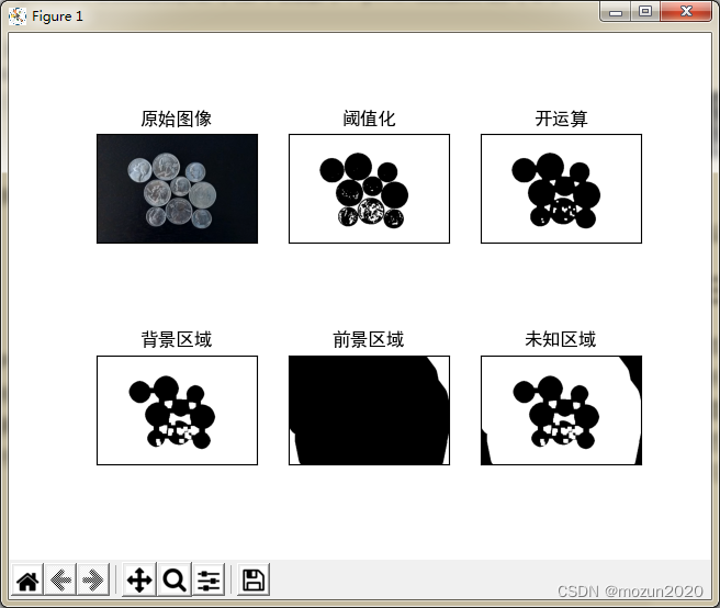
#图像开运算消除噪声
kernel = np.ones((3,3),np.uint8)
opening = cv2.morphologyEx(thresh,cv2.MORPH_OPEN,kernel, iterations = 2)

#图像膨胀操作确定背景区域
sure_bg = cv2.dilate(opening,kernel,iterations=3)

#距离运算确定前景区域
dist_transform = cv2.distanceTransform(opening,cv2.DIST_L2,5)
ret, sure_fg = cv2.threshold(dist_transform, 0.7*dist_transform.max(), 255, 0)

#寻找未知区域
sure_fg = np.uint8(sure_fg)
unknown = cv2.subtract(sure_bg, sure_fg)

#用来正常显示中文标签
plt.rcParams['font.sans-serif']=['SimHei']

#显示图像
titles = [u'原始图像', u'阈值化', u'开运算',
          u'背景区域', u'前景区域', u'未知区域']  
images = [img, thresh, opening, sure_bg, sure_fg, unknown]  
for i in range(6):  
   plt.subplot(2,3,i+1), plt.imshow(images[i], 'gray')  
   plt.title(titles[i])  
   plt.xticks([]),plt.yticks([])  
plt.show()

保存.py文件输入以下命令，跑起工程

python chapter14_10.py

没有报错，直接弹出图片，运行成功！

三. 小结

本文主要介绍在Python中调用OpenCV库对图像进行分割，如k-means聚类分割，均值漂移分割，阈值分割等。由于本书的介绍比较系统全面，所以会出一个系列文章进行全系列仿真实现，下一篇文章将继续介绍第十四章节的最后4例仿真实例，感兴趣的还是建议去原书第十四章深入学习理解。每天学一个Python小知识，大家一起来学习进步阿！

本系列示例主要参考杨老师GitHub源码，安利一下地址：ImageProcessing-Python（喜欢记得给个star哈！）