通过领域滤波（卷积）来实现图像滤镜效果

这篇文章中主要是通过python对卷积的滤镜效果实现，在性能上并未做任何优化。如果对滤镜的调用感兴趣的朋友可以直接参考代码后面部分图像滤镜函数的调用

===================================================================================

领域算子是利用给定像素周围的像素值决定此像素的最终输出值。领域算子除了用于局部色调调整还可以用于图像滤波，实现图像的平滑和锐化，图像边缘的增强或者图像噪声的去除

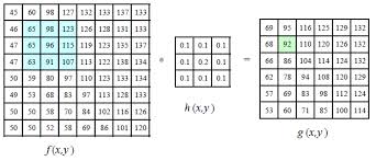
如上图所示算子h(x,y)对图像f(x,y)中的(1,1)~(3,3)区域进行卷积操作得到新图像g(x,y)上(1,1)上的图像信息，这里的卷积是指的算子h(x,y)中每个元素与图像f(x,y)中某块大小一致的区域进行一对一的乘操作并将结果累加作为新图像的结果，具体公式如下：

有了以上基础概念就可以开始代码实现的工作了，这里先介绍下已有的图像滤镜函数

#模糊
imgfilted = im_source.filter(ImageFilter.BLUR)
#轮廓
imgfilted = im_source.filter(ImageFilter.CONTOUR)
#边缘增强
imgfilted = im_source.filter(ImageFilter.EDGE_ENHANCE)
imgfilted = im_source.filter(ImageFilter.EDGE_ENHANCE_MORE)
#浮雕
imgfilted = im_source.filter(ImageFilter.EMBOSS)
imgfilted = im_source.filter(ImageFilter.FIND_EDGES)
#平滑
imgfilted = im_source.filter(ImageFilter.SMOOTH)
imgfilted = im_source.filter(ImageFilter.SMOOTH_MORE)
imgfilted = im_source.filter(ImageFilter.SHARPEN)

以上代码的调用可以参考PIL中ImageFilter

以下就是卷积操作的核心代码这里函数参数分别为imdata图像数据，opedata算子数据，offset操作结果的偏移量

# 卷积函数,卷积算子为3*3或5*5矩阵
def convolution(imdata, opedata, offset=0, packing=None):
    end_w = len(imdata[0])
    end_h = len(imdata)
    start_w = 0
    start_h = 0
    run_start_w = 0

    # 算子宽度
    opedata_w = len(opedata[0])
    opedata_h = len(opedata)
    
    if packing == None:
        run_start_w = math.floor(opedata_w/2)
        end_w -= run_start_w
        end_h -= run_start_w
        start_w = run_start_w
        start_h = run_start_w
        pass

    im_result = []
    while start_h < end_h:
        im_line = []
        while start_w < end_w :
            # 开始卷积操作
            step_w = step_h = 0
            r = g = b = 0
            while step_h < opedata_h:
                while step_w < opedata_w:
                    p_r, p_g, p_b = imdata[start_h+step_h-run_start_w][start_w+step_w-run_start_w]
                    op_v   = opedata[step_h][step_w]
                    r += p_r*op_v
                    g += p_g*op_v
                    b += p_b*op_v
                    step_w += 1
                    pass
                step_h += 1
                step_w = 0
                pass

            r = min(max(int(r + offset), 0), 255)
            g = min(max(int(g + offset), 0), 255)
            b = min(max(int(b + offset), 0), 255)
            
            im_line.append([r, g, b])
            start_w += 1
        pass

        im_result.append(im_line)
        start_h += 1
        start_w = run_start_w
    pass

    return im_result

如果你看完代码可能会有这样的疑问，如果一个100×100的图像在操作完成后会变为一个98×98的图像这样的操作会影响图像的大小。这里确实没有对空缺的外围像素做补全，当然对应的算法还是比较多比如用算子中心对应的图像做补全，用所有有效像素均值补全，用最靠近的像素补全等方式。

第二个问题主要是对于性能，这里用3×3的算子进行运算时速度还可以忍受5×5就明显感觉很慢了，如果对于更大的算子其速度将会是算子直径的平方来n^2增加这对大算子来说是不能忍受的。解决这个问题的方法是使用奇异值分解也就是说可以可以将目前的2维核分解为水平方向和垂直方向的两个卷积这样运算复杂度可以降为2n。

当你对卷积计算完成后由于结果有可能会超出图像应有的范围值如：<0 or >255，再有可能由于不同的算子特点可能需要给值增加一个偏移值所以需要对结果进行修正

r = min(max(int(r + offset), 0), 255)
g = min(max(int(g + offset), 0), 255)
b = min(max(int(b + offset), 0), 255)

之后就可以将结果放到一个新的图像内了，下面是完整的调用代码：

# -*-  coding: utf-8 -*-
# 线性滤波例子

from PIL import Image, ImageFilter
from numpy import *
#from matplotlib import pyplot
from scipy.misc import lena, toimage
from pylab import *
import math


# 卷积函数,卷积算子为3*3或5*5矩阵
def convolution(imdata, opedata, offset=0, packing=None):
    end_w = len(imdata[0])
    end_h = len(imdata)
    start_w = 0
    start_h = 0
    run_start_w = 0

    # 算子宽度
    opedata_w = len(opedata[0])
    opedata_h = len(opedata)
    
    if packing == None:
        run_start_w = math.floor(opedata_w/2)
        end_w -= run_start_w
        end_h -= run_start_w
        start_w = run_start_w
        start_h = run_start_w
        pass

    im_result = []
    while start_h < end_h:
        im_line = []
        while start_w < end_w :
            # 开始卷积操作
            step_w = step_h = 0
            r = g = b = 0
            while step_h < opedata_h:
                while step_w < opedata_w:
                    p_r, p_g, p_b = imdata[start_h+step_h-run_start_w][start_w+step_w-run_start_w]
                    op_v   = opedata[step_h][step_w]
                    r += p_r*op_v
                    g += p_g*op_v
                    b += p_b*op_v
                    step_w += 1
                    pass
                step_h += 1
                step_w = 0
                pass

            r = min(max(int(r + offset), 0), 255)
            g = min(max(int(g + offset), 0), 255)
            b = min(max(int(b + offset), 0), 255)
            
            im_line.append([r, g, b])
            start_w += 1
        pass

        im_result.append(im_line)
        start_h += 1
        start_w = run_start_w
    pass

    return im_result

if __name__ == '__main__':
    im_source = Image.open('images/902127300357814245.jpg')
    arr_im_source = array(im_source);
    w = len(arr_im_source[0])
    h = len(arr_im_source)
    im_half_source = im_source.resize([w/6, h/6])
    arr_im_source = array(im_half_source);

    if False:
        imgfilted = im_source.filter(ImageFilter.BLUR)
        imgfilted.show()
        imgfilted = im_source.filter(ImageFilter.CONTOUR)
        imgfilted.show()
        imgfilted = im_source.filter(ImageFilter.EDGE_ENHANCE)
        imgfilted.show()
        imgfilted = im_source.filter(ImageFilter.EDGE_ENHANCE_MORE)
        imgfilted.show()
        imgfilted = im_source.filter(ImageFilter.EMBOSS)
        imgfilted.show()
        imgfilted = im_source.filter(ImageFilter.FIND_EDGES)
        imgfilted.show()
        imgfilted = im_source.filter(ImageFilter.SMOOTH)
        imgfilted.show()
        imgfilted = im_source.filter(ImageFilter.SMOOTH_MORE)
        imgfilted.show()
        imgfilted = im_source.filter(ImageFilter.SHARPEN)
        imgfilted.show()
        exit()

    # 设置卷积算子
    # 模糊效果
    operator1 = [[0.1, 0.1, 0.1],[0.1, 0.2, 0.1], [0.1, 0.1, 0.1]]
    # 高斯模糊
    operator2 = [[1.0/256, 4.0/256, 6.0/256, 4.0/256, 1.0/256],
                 [4.0/256, 16.0/256, 24.0/256, 16.0/256, 4.0/256],
                 [6.0/256, 24.0/256, 36.0/256,  24.0/256, 6.0/256],
                 [4.0/256, 16.0/256, 24.0/256, 16.0/256, 4.0/256],
                 [1.0/256, 4.0/256, 6.0/256, 4.0/256, 1.0/256]]
    # 角点
    operator3 = [[0.25, -0.5, 0.25], [-0.5, 1, -0.5], [0.25, -0.5, 0.25]]
    # Sobel
    operator4 = [[-0.125, 0, 0.125], [-0.25, 0, 0.25], [-0.125, 0, 0.125]]
    operator5 = [[0, 1, 0], [1, -4, 1], [0, 1, 0]]

    # 对于Sobel过滤各点和值为零，所以将偏移量设为128
    #convert_im = convolution(arr_im_source, operator4, 128)
    convert_im = convolution(arr_im_source, operator5)
    arr_im_half = array(im_half_source)

    figure()
    imShow = toimage(array(convert_im), 255)
    imShow.show()
    im_half_source.show()

由于用python来实现确实性能比较差，而且也没有做过性能优化所以在处理原图的时候直接先缩小到1/6再来处理。

对于第四个算子由于其算子各部分和为0所以需要将偏移量设为128，不然你将会看到大片的黑色。

最后附上处理后图像的不同效果

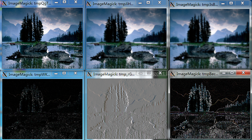
第一行分别是原图，平滑模糊，高斯模糊，第二行分别是角点，Sobel。

通过领域滤波（卷积）来实现图像滤镜效果

猜你喜欢