URP SMAA 细品
“这咋和书上的不一样呢!“
虽然,标题挂了一个URP,实际上本文主要是对SMAA算法做出说明,Unity 只是一个实验验证的工具。在URP中涉及到SMAA的主要地方如下:
SubpixelMorphologicalAntialiasing.shaderSubpixelMorphologicalAntialiasingBridge.hlslSubpixelMorphologicalAntialiasing.hlsl
这里我们重点关注最后一个,它和Github项目:SMAA 中的 SMAA.hlsl大体上是一致的。
阅读注意:
- 本文目前暂时只涉及到 SMAA 1x 的内容。
- 本文的URP 版本为 10.8.1
1 SMAA 大致思路
SMAA 是基于形态的抗锯齿算法,它会将锯齿的边缘形状类型分类,对不同的边缘形状样式有着不同的计算方式。例如现在有一个锯齿边缘如下:

注意蓝色边缘,让这个成为了一个形状类似字母Z的 Z型 Pattern 锯齿边缘。那么,我们可以规定,这类锯齿是由下图中红色原始边缘光栅化而来。所以我们需要**重新矢量化(re-vectorizing)**轮廓来得到被“锯齿化“的原始边缘。

如果得到了原始边缘,那就好办了。你只需要一点点计算,将蓝色水平线和红色原始边缘的覆盖面积算出来。以蓝色水平线为基准,覆盖面积在蓝线之上的,颜色往上混合,反之,颜色往下混合。混合比例为覆盖面积占像素面积的比例。

该算法思路还是蛮朴素的,只要定好了不同边缘样式的混合比例计算方式,反锯齿的效果就有保证了。
该算法分为了三个流程:
- 边缘检测
- 边缘的模式检测和覆盖区域的计算
- 根据混合比例进行混合
Unity 也将其实现为了对应的三个Pass。
2 SMAA 具体实现流程
由于代码实在太多,我们只关注SubpixelMorphologicalAntialiasing.hlsl或 SMAA.hlsl中的内容。
2.1 边缘检测
2.1.1 顶点着色器 SMAAEdgeDetectionVS
我们首先来康康边缘检测的顶点着色器。
/**
 * Edge Detection Vertex Shader
 */
void SMAAEdgeDetectionVS(float2 texcoord,
                         out float4 offset[3]) {


    offset[0] = mad(SMAA_RT_METRICS.xyxy, float4(-1.0, 0.0, 0.0, -1.0), texcoord.xyxy);
    offset[1] = mad(SMAA_RT_METRICS.xyxy, float4( 1.0, 0.0, 0.0,  1.0), texcoord.xyxy);
    offset[2] = mad(SMAA_RT_METRICS.xyxy, float4(-2.0, 0.0, 0.0, -2.0), texcoord.xyxy);
}
其中:
SMAA_RT_METRICS填充了待反走样贴图(屏幕贴图)的尺寸数据(1/width, 1/height, width, height)
代码中出现了一个mad函数,这是一种优化的手段,具体请看官方文档 mad 。它的作用是先乘后加,mad(m, a, b) 的作用 和 m * a + b 一致。
这段代码将几个偏移数据存放在了offset[3]中,如下图所示:

注意:在Direct3D中UV是上下翻转的,y轴上-1是向上偏移。
至于这几个偏移数据怎么用,我们继续往后看。
2.1.2 片元着色器 SMAAColorEdgeDetectionPS
我们看向片元着色器
/**
 * Color Edge Detection
 *
 * IMPORTANT NOTICE: color edge detection requires gamma-corrected colors, and
 * thus 'colorTex' should be a non-sRGB texture.
 */
float2 SMAAColorEdgeDetectionPS(float2 texcoord,
    float4 offset[3],
    SMAATexture2D(colorTex)
#if SMAA_PREDICATION
    , SMAATexture2D(predicationTex)
#endif
) {


...
}
其中:
colorTex:待处理的屏幕贴图SMAA_PREDICATION:这是一个可选的宏定义,开启时,会使用predicationTex来预测边缘检测的阈值,否则阈值是一个固定值。当前URP版本并未开启此选项。
这里插一句,边缘检测的函数一共提供了三种:亮度、颜色或深度。在SMAA.hlsl中它这样解释到:
- 深度边缘检测最快,但可能会错误一些边缘
- 亮度边缘检测通常比深度更耗费性能,但能捕获到一些深度检测捕获不到的可见边缘
- 颜色边缘检测是最耗费性能的,它能捕获一些色度(chroma-only edge)上的边缘。
当前URP中默认使用的以颜色边缘检测的方法。
好了,我们继续往下看:
#if SMAA_PREDICATION
float2 threshold = SMAACalculatePredicatedThreshold(texcoord, offset, predicationTex);
#else
float2 threshold = float2(SMAA_THRESHOLD, SMAA_THRESHOLD);
#endif
SMAA_THRESHOLD根据反走样品质而变化,默认情况下,最高品质为0.05,最低品质为0.15
阈值这里由宏定义SMAA_PREDICATION分为了相对阈值和绝对阈值。不着急,我们先来看看绝对阈值,最后再回头来看相对阈值。
// Calculate color deltas:
float4 delta;
float3 C = PositivePow(SMAASamplePoint(colorTex, texcoord).rgb, GAMMA_FOR_EDGE_DETECTION);

float3 Cleft = PositivePow(SMAASamplePoint(colorTex, offset[0].xy).rgb, GAMMA_FOR_EDGE_DETECTION);
float3 t = abs(C - Cleft);
delta.x = max(max(t.r, t.g), t.b);

float3 Ctop = PositivePow(SMAASamplePoint(colorTex, offset[0].zw).rgb, GAMMA_FOR_EDGE_DETECTION);
t = abs(C - Ctop);
delta.y = max(max(t.r, t.g), t.b);

// We do the usual threshold:
float2 edges = step(threshold, delta.xy);

// Then discard if there is no edge:
if (dot(edges, float2(1.0, 1.0)) == 0.0)
    discard;
GAMMA_FOR_EDGE_DETECTION:这是Unity自己加上去的,和Unity的颜色空间有关,在Gamma空间下为1,在Linear空间下为1/2.2
这一段和SMAA.hlsl有点不同,在Linear空间下,Unity采样完后,进行了一次颜色校正,让颜色位于Gamma 0.45 空间下。说实话,这里我有点不明白,注释中”requires gamma-corrected colors“和” non-sRGB texture“的具体原因。不过在sRGB空间下,应该可以检测到更多人眼可以观察到的边缘。
上面这段,我们计算了当前位置与左边和上边的颜色差值,选取RGB通道中最大的差值绝对值,分别存放在delta的xy中。如果两个方向上,有任意一方向这个差值超过了阈值threshold,就说明在这个方向上存在边缘。edges是一个二维向量,其中R通道存放左边的边缘信息,G通道存放顶部的边缘信息,值为1,则说明当前方向上存在边缘。那么可以生成贴图如下:

按理说,边缘检测部分可以到此结束,但SMAA算法大佬们意识到这样做有一个缺点,它默认了边缘是一个二进制的概念,要么有要么没有,有时候边缘的轮廓是可能存在渐变的。
由于”人类视觉系统倾向于在周围区域存在更高对比度的情况下掩盖低对比度边缘“,上图中虽然水平方向上的对比度变化较大,但它明显不如垂直方向上变化来得大,所以红色标记部分不应该是边缘。
为了解决这个问题,我们还需要进行局部对比度适应(Local contrast adaptation)。
    // Calculate right and bottom deltas:
    float3 Cright = PositivePow(SMAASamplePoint(colorTex, offset[1].xy).rgb, GAMMA_FOR_EDGE_DETECTION);
    t = abs(C - Cright);
    delta.z = max(max(t.r, t.g), t.b);

    float3 Cbottom = PositivePow(SMAASamplePoint(colorTex, offset[1].zw).rgb, GAMMA_FOR_EDGE_DETECTION);
    t = abs(C - Cbottom);
    delta.w = max(max(t.r, t.g), t.b);

    // Calculate the maximum delta in the direct neighborhood:
    float2 maxDelta = max(delta.xy, delta.zw);

    // Calculate left-left and top-top deltas:
    float3 Cleftleft = PositivePow(SMAASamplePoint(colorTex, offset[2].xy).rgb, GAMMA_FOR_EDGE_DETECTION);
    t = abs(Cleft - Cleftleft);
    delta.z = max(max(t.r, t.g), t.b);

    float3 Ctoptop = PositivePow(SMAASamplePoint(colorTex, offset[2].zw).rgb, GAMMA_FOR_EDGE_DETECTION);
    t = abs(Ctop - Ctoptop);
    delta.w = max(max(t.r, t.g), t.b);

    // Calculate the final maximum delta:
    maxDelta = max(maxDelta.xy, delta.zw);
    float finalDelta = max(maxDelta.x, maxDelta.y);

    // Local contrast adaptation:
#if !defined(SHADER_API_OPENGL)
    edges.xy *= step(finalDelta, SMAA_LOCAL_CONTRAST_ADAPTATION_FACTOR * delta.xy);
#endif

    return edges;
SMAA_LOCAL_CONTRAST_ADAPTATION_FACTOR:默认情况为2.0
这里还计算了当前点O 与右侧点C、底部点D、顶部的顶部点F、左侧的左侧点E的颜色差值,并通过比较获得了它们之间的最大差值maxDelta,即计算了周围最大的对比度增量。以左边缘为例,如果左边缘差值delta.x高于最大差值maxDelta的一定比例,边缘就会被保留,这里这个比例在这里是0.5(SMAA_LOCAL_CONTRAST_ADAPTATION_FACTOR默认值为2.0)。
最后,所有边缘信息被保存在了一张名为edgesTex的贴图中。
2.1.3 绝对阈值与相对阈值
Playstation EDGE MLAA 团队提出了一种相对阈值的方法,它允许通过一张额外的材质,找到边缘并降低当前的亮度或颜色阈值。
/**
 * Gathers current pixel, and the top-left neighbors.
 */
float3 SMAAGatherNeighbours(float2 texcoord,
    float4 offset[3],
    SMAATexture2D(tex)) {


#ifdef SMAAGather
    return SMAAGather(tex, texcoord + SMAA_RT_METRICS.xy * float2(-0.5, -0.5)).grb;
#else
    float P = SMAASamplePoint(tex, texcoord).r;
    float Pleft = SMAASamplePoint(tex, offset[0].xy).r;
    float Ptop = SMAASamplePoint(tex, offset[0].zw).r;
    return float3(P, Pleft, Ptop);
#endif
}

/**
 * Adjusts the threshold by means of predication.
 */
float2 SMAACalculatePredicatedThreshold(float2 texcoord,
    float4 offset[3],
    SMAATexture2D(predicationTex)) {


    float3 neighbours = SMAAGatherNeighbours(texcoord, offset, SMAATexturePass2D(predicationTex));
    float2 delta = abs(neighbours.xx - neighbours.yz);
    float2 edges = step(SMAA_PREDICATION_THRESHOLD, delta);
    return SMAA_PREDICATION_SCALE * SMAA_THRESHOLD * (1.0 - SMAA_PREDICATION_STRENGTH * edges);
}
SMAA_PREDICATION_THRESHOLD:用在predicationTex上的阈值,默认为0.01SMAA_PREDICATION_SCALE:对全局阈值的缩放,默认为 2.0SMAA_THRESHOLD:全局阈值,具体值由反走样品质而定SMAA_PREDICATION_STRENGTH:局部阈值降低多少
这里的predicationTex我们可以传入一张深度图为例。获取顶部和左边的深度差,超过预测阈值识别为边缘,然后根据边缘信息对全局阈值进行调整。

2.2 边缘模式检测和覆盖区域计算
2.2.1 边缘模式检测
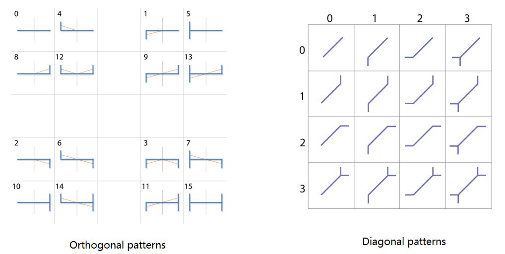
我们拿到了边缘信息贴图edgesTex,通过它我们可以获取当前像素的上边界和左边界信息。在大致思路那里说了,现在我们的首要任务时确认边缘的样式,然后按照样式进行混合比例的计算。SMAA作者将边缘类型分为了两个大类,一个为正交方向上的边缘样式(orthogonal patterns),另一个是对角线方向上的边缘样式(diagonal patterns)。每个大类各罗列16种类型,如下图所示:
我们先以正交方向的样式4为例,确认一个样式的方法是比较土味的,以下图为例:
 当前的采样点 O O O在像素点中心,我们只需要对
edgesTex进行搜索:
- 向左搜索:每次向左偏移一个像素的距离,直到搜索到点 A A A。由于上边的点 B B B拥有左边缘,点 A A A拥有上边缘,构成了一个
L型(注意蓝色边)的交叉边(crossing edges)。 - 向右搜索:每次向右偏移一个像素的距离,直到超出搜索范围,都没出现交叉边。
综合确认这是一个样式4的边缘类型。
又比如说样式1:

向左搜索到 A A A点时,发现同时存在上边界和左边界,构成倒L型交叉边;向右搜索,直到超出范围都没有交叉边。综合说明这是一个样式1的边缘类型。
这里我们确认了一件事,为了正交方向的边缘类型,搜索时需要同时检查采样点所在行和采样点上边像素行,一共两行的边缘信息。

可以想象,如果老老实实按照每次移动一个像素距离,采样像素点中心的方式,确认一次边缘类型会进行大量的采样。那么,有没有什么方法可以减少采样次数呢?
2.2.2 双线性过滤 Bilinear Filtering
双线性过滤将会在后续多个地方被使用,如果没有充分理解,后面的代码可能真就如同魔法一样难以理解。所以在正式开始之前,我们有必要了解一下这项技术。度娘解释如下:
双线性过滤(Bilinear_filtering)是进行缩放显示的时候进行纹理平滑的一种纹理过滤方法。 在大多数情况下,纹理在屏幕上显示的时候都不会同保存的纹理一模一样,没有任何失真。正因为这样,所以一些像素要使用纹素之间的点进行表示,在这里我们假设纹素都是位于各个单元中心或者左上或者其它位置的点。双线性过滤器利用这些点在像素所表示点周围四个最近的点之间进行双线性插值。
简单地说,当前纹理坐标如果和像素中心不完全对齐时,我们会取离这一点最近的四个像素点,并对它们进行双线性插值,算出当前坐标的值。
我们先从简单的线性插值开始,假设这里有两个像素点 a a a和 b b b,采样点 c c c位于两点之间,距离 a c ac ac占总距离 a b ab ab的比例为 x x x。

采样点 c c c处的值 V c V_c Vc可表示为:
V c = ( 1 − x ) V a + x V b V_c=(1-x)V_a+xV_b Vc=(1−x)Va+xVb
有意思的事情发生了,如果 V a V_a Va和 V b V_b Vb的值只能从0和1中选的话, V c V_c Vc和它们构成了如下关系:
| V a V_a Va | V b V_b Vb | V c V_c Vc |
|---|---|---|
| 0 | 0 | 0 |
| 0 | 1 | x x x |
| 1 | 0 | 1 − x 1-x 1−x |
| 1 | 1 | 1 |
如果 x ≠ 0.5 x\neq0.5 x=0.5, V a V_a Va、 V b V_b Vb和 V c V_c Vc构成了一一对应关系,那么仅靠采样点的值 V c V_c Vc的值就能推出 V a V_a Va和 V b V_b Vb的值!!!这意味着原本我需要采样两次才能获得的值,我现在一次采样就能获得。
但很明显这还只是在一维空间上的情况,我们试试在二维空间上进行双线性插值。

采样点值 V e V_e Ve可表示为:
V e = x y V a + ( 1 − x ) y V b + x ( 1 − y ) V c + ( 1 − x ) ( 1 − y ) V d V_e=xyV_a + (1-x)yV_b + x(1-y)V_c + (1-x)(1-y)V_d Ve=xyVa+(1−x)yVb+x(1−y)Vc+(1−x)(1−y)Vd
同样,当周围点的取值只有0和1时,只靠 V c V_c Vc值也能推出参与插值的四个点的值。为了方便后续说明,我这里直接取 x = 0.25 x=0.25 x=0.25和 y = 0.125 y=0.125 y=0.125。
| V a V_a Va | V b V_b Vb | V c V_c Vc | V d V_d Vd | V e V_e Ve |
|---|---|---|---|---|
| 0 | 0 | 0 | 0 | 0.0 |
| 0 | 0 | 0 | 1 | 0.65625 |
| 0 | 0 | 1 | 0 | 0.21875 |
| 0 | 0 | 1 | 1 | 0.875 |
| 0 | 1 | 0 | 0 | 0.09375 |
| 0 | 1 | 0 | 1 | 0.75 |
| 0 | 1 | 1 | 0 | 0.3125 |
| 0 | 1 | 1 | 1 | 0.96875 |
| 1 | 0 | 0 | 0 | 0.03125 |
| 1 | 0 | 0 | 1 | 0.9875 |
| 1 | 0 | 1 | 0 | 0.25 |
| 1 | 0 | 1 | 1 | 0.90625 |
| 1 | 1 | 0 | 0 | 0.125 |
| 1 | 1 | 0 | 1 | 0.78125 |
| 1 | 1 | 1 | 0 | 0.34375 |
| 1 | 1 | 1 | 1 | 1.0 |
现在对于像edgesTex这样材质(前提是纹理开启双线性插值),我们需要偏移合适的值,就能一次采样获取附近四个像素点的值了!我们以下图为例:

向左搜索时,我们从点 O O O纹理坐标偏移(-0.25,-0.125)的点 L 0 L_0 L0开始,采样edgesTex获得一个二维向量 e ( r , g ) e(r,g) e(r,g)。那么,确认此处周围没有交叉边且可以继续往左搜索的条件是什么呢?我们将 L 0 L_0 L0涉及到的周围四个像素截出来:

条件有两个:
- e . r = = 0 e.r==0 e.r==0 :周围四个像素都不能拥有左边界,否则此处存在交叉边,所以插值出来的 e . r e.r e.r必须为0。
- e . g > 0.8281 e.g>0.8281 e.g>0.8281:为了保证没有交叉边且可以继续往左搜索,周围四个像素的底下两个必须拥有上边界,即必须 e . g > = 0.875 e.g >= 0.875 e.g>=0.875。但在实际操作过程中,我们还要取小于0.875的最大插值结果0.78125,用它们做一个平均(可能这样比较稳),将边界条件设置为0.8281( ( 0.875 + 0.78125 ) / 2 (0.875 + 0.78125)/2 (0.875+0.78125)/2)。
只要满足以上两个条件,就将采样点往左移动两个像素单位,对点 L 1 L_1 L1进行采样。

很明显,由于点 B B B拥有左边界,插值出来的 e . r ≠ 0 e.r\neq0 e.r=0,此处存在交叉边,停止搜索。在这里我们需要明确四个像素的具体值,才能判断交叉边到底出现在哪个地方,这个边缘到底是哪个样式。
那么,这个四个具体的值怎么得到呢?我们可以依据之前的双线性插值表,一一对应查找。但仔细一想,对于一个插值结果,在最糟糕的情况下,需要判断15次才能确定四个像素点的值,这也太拉了。我们需要一个更好的方法,让它能够一次性就干出来。
(往右搜索也是同样的道理,不过起点 R 0 R_0 R0的偏移值是(1.25,-0.125))
2.2.3 SearchTex
为了更好地在搜索的最后一步确认交叉边的位置,现在开始我们要制作一张材质SearchTex。以下的Python代码出自SearchTex.py,这里只对关键位置做出说明。
# Interpolates between two values:
def lerp(v0, v1, p):
    return v0 + (v1 - v0) * p

# Calculates the bilinear fetch for a certain edge combination:
def bilinear(e):
    # e[0]       e[1]
    #
    #          x <-------- Sample position:    (-0.25,-0.125)
    # e[2]       e[3] <--- Current pixel [3]:  (  0.0, 0.0  )
    a = lerp(e[0], e[1], 1.0 - 0.25)
    b = lerp(e[2], e[3], 1.0 - 0.25)
    return lerp(a, b, 1.0 - 0.125)

# This dict returns which edges are active for a certain bilinear fetch:
# (it's the reverse lookup of the bilinear function)
edge = {


    bilinear([0, 0, 0, 0]): [0, 0, 0, 0],
    bilinear([0, 0, 0, 1]): [0, 0, 0, 1],
    bilinear([0, 0, 1, 0]): [0, 0, 1, 0],
    bilinear([0, 0, 1, 1]): [0, 0, 1, 1],

    bilinear([0, 1, 0, 0]): [0, 1, 0, 0],
    bilinear([0, 1, 0, 1]): [0, 1, 0, 1],
    bilinear([0, 1, 1, 0]): [0, 1, 1, 0],
    bilinear([0, 1, 1, 1]): [0, 1, 1, 1],

    bilinear([1, 0, 0, 0]): [1, 0, 0, 0],
    bilinear([1, 0, 0, 1]): [1, 0, 0, 1],
    bilinear([1, 0, 1, 0]): [1, 0, 1, 0],
    bilinear([1, 0, 1, 1]): [1, 0, 1, 1],

    bilinear([1, 1, 0, 0]): [1, 1, 0, 0],
    bilinear([1, 1, 0, 1]): [1, 1, 0, 1],
    bilinear([1, 1, 1, 0]): [1, 1, 1, 0],
    bilinear([1, 1, 1, 1]): [1, 1, 1, 1],
}
代码刚开始,就做了和我们之前做过的事,将(-0.25,-0.125)偏移的双线性插值结果和参与插值的四个像素值一一对应,起来保存在了edge中。
再次观察一下,之前给出的16个插值结果,它们之间其实有一个最大公约数0.03125,可以把1分 1 / 0.03125 + 1 = 33 1/0.03125+1=33 1/0.03125+1=33份(端点也算一份)。那么,我们可以把从edgeTex插值采样出来的值作为一个新的UV坐标,去采样一个33x33的材质。
# Calculate delta distances to the left:
image = Image.new("RGB", (66, 33))
for x in range(33):
    for y in range(33):
        texcoord = 0.03125 * x, 0.03125 * y
        if texcoord[0] in edge and texcoord[1] in edge:
            edges = edge[texcoord[0]], edge[texcoord[1]]
            val = 127 * deltaLeft(*edges) # Maximize dynamic range to help compression
            image.putpixel((x, y), (val, val, val))
            #debug("left: ", texcoord, val, *edges)

# Calculate delta distances to the right:
for x in range(33):
    for y in range(33):
        texcoord = 0.03125 * x, 0.03125 * y
        if texcoord[0] in edge and texcoord[1] in edge:
            edges = edge[texcoord[0]], edge[texcoord[1]]
            val = 127 * deltaRight(*edges) # Maximize dynamic range to help compression
            image.putpixel((33 + x, y), (val, val, val))
            #debug("right: ", texcoord, val, *edges)
由于向左搜索和向右搜索情况不同,代码将材质大小设为了66x33。材质左半部分供向左搜索的采样,右半部分供向右搜索的采样。代码枚举了所有像素中心位置的UV,如果这个UV是双线性插值结果能够组合出来的,就对当前像素位置填充值val。这个Val由两个函数计算deltaLeft和deltaRight。
# Delta distance to add in the last step of searches to the left:
def deltaLeft(left, top):
    d = 0

    # If there is an edge, continue:
    if top[3] == 1:
        d += 1

    # If we previously found an edge, there is another edge and no crossing
    # edges, continue:
    if d == 1 and top[2] == 1 and left[1] != 1 and left[3] != 1:
        d += 1

    return d
传入的left和top数组,我们可以想成参与插值的四个像素的左边界信息和上边界信息。当top[3](右下)有上边界时,交叉边在距离右侧 d = 1 d=1 d=1的位置;当top[2]和top[3](左下和右下)均有上边界,且left[1]和left[3](右上和右下)没有左边界时,交叉边在距离右侧 d = 2 d=2 d=2的位置;否则,交叉边就在最右侧, d = 0 d=0 d=0。

d d d可取的值为0、1和2,将它乘以127映射为0、127和254,并填入到SearchTex当中。 (deltaRight同理)

在后续的代码中,作者去除了上面大量黑色部分,将图片裁剪为了64x16,与2的n次幂对齐。
# Crop it to power-of-two to make it BC4-friendly:
# (Cropped area and borders are black)
image = image.crop([0, 17, 64, 33])
image = image.transpose(Image.FLIP_TOP_BOTTOM)
emmmmm,不过不知为何,作者还对其进行了翻转。URP中的SearchTex存放在Packages\Universal RP\Textures\SMAA文件夹下,如下所示:

可以看到URP并未对其进行翻转。
有了这张材质,我们在搜索edgesTex最后一步时,就能很轻松的锁定交叉边的位置(SearchTex只在正交方向的搜索中使用,对角方向判断逻辑相对来说更加直接),具体采样细节后面结合代码谈。
2.2.4 AreaTex
千万被忘了,我们做这么多的事情的目的是什么!!!我们需要确认边界样式!知道了交叉边位置又如何确定?
例如,在向左搜索到末尾时,你知道交叉边在最后 d = 2 d=2 d=2的地方,但它的实际情况可分为以下几类(只取了几个代表):

没错,我们还要在边界附近确认上下两个像素的左边界情况,你大可以采样两次来确认。但我们依旧采用插值的方式,一次采样获取两个点的信息。注意,这里只需要将采样点向上偏移0.25就行了,没必要偏移x轴牵扯进没必要的像素。

采样点 L 2 L_2 L2就是我们向左搜索过程中最后的采样点(最左端向上偏移采样),不同的左边界情况采样得到的值有如下几种情况(只看R通道):

用下图做演示,我们设最左端的距离 O A OA OA为 d l d_l dl,最后偏移采样点 L 2 L_2 L2获得的值为 e 1 e_1 e1;最右端的距离 O C OC OC为 d r d_r dr,最后偏移采样点 R 2 R_2 R2获得的值为 e 2 e_2 e2,

这整个边界样式可以用 ( e 1 . r , e 2 . r ) (e_1.r,e_2.r) (e1.r,e2.r)概括,例如:样式0为(0,0)、样式4为(0.25,0)、样式12为(0.25,0.25)等。
每个分量的范围都在 [ 0 , 1 ] [0,1] [0,1]范围内!如果你足够敏锐,你应该猜到接下来要发生什么了!
没错,我们可以建立一张材质AreaTex,这张材质可通过 ( e 1 . r , e 2 . r ) (e_1.r,e_2.r) (e1.r,e2.r)锁定到专属于该边缘样式的局部区域,在这个局部区域内,我们可以通过 ( d l , d r ) (d_l,d_r) (dl,dr)去查到该像素的混合比例。

好了,说了这么多,我们直接来品鉴一下AreaTex材质的生成代码,以下Python代码来自于AreaTex.py,同样这里只对关键代码进行说明。
# Texture sizes:
# (it's quite possible that this is not easily configurable)
SIZE_ORTHO = 16 # * 5 slots = 80
SIZE_DIAG  = 20 # * 4 slots = 80
由于有正交方向和对角方向的边缘,我们会创建两个80x80的大小的材质。
2.2.4.1 正交方向
我们还是先说正交方向,SIZE_ORTHO为16代表每个边缘模式的占用的局部区域大小为16x16,乘以5是因为最后采样点采到的值可能有0、0.25、0.75和1,1由最大公约数0.25刚好划分为5份(事实上0.5是无法取得的,所以正交方向生成的贴图中间会有一个黑色十字架)。
# Creates a 2D orthogonal pattern subtexture:
def tex2dortho(args):
    pattern, path, offset = args
    size = (SIZE_ORTHO - 1)**2 + 1
    tex2d = Image.new("RGBA", (size, size))
    for y in range(size):
        for x in range(size):
            p = areaortho(pattern, x, y, offset)
            p = p[0], p[1], 0.0, 0.0
            tex2d.putpixel((x, y), bytes(p))
    tex2d.save(path, "TGA")
pattern:指16个边缘类型,取值0到15offset:SMAA 1x默认此值为0,不多说
这里将局部大小平方了一下,最后输出的时候还是会压缩为SIZE_ORTHO。
这段代码采用暴力法遍历材质的每一个像素点,x为该像素距离左边界的距离,y为距离右边界的距离,以此为依据,在areaortho中计算混合比例。
# Horizontal/Vertical Areas

# Calculates the area for a given pattern and distances to the left and to the
# right, biased by an offset:
def areaortho(pattern, left, right, offset):

	... area 面积计算

    # o1           |
    #      .-------´
    # o2   |
    #
    #      <---d--->
    d = left + right + 1

    o1 = 0.5 + offset
    o2 = 0.5 + offset - 1.0

    if pattern == 0:
        #
        #    ------
        #
        return 0.0, 0.0

    ...其他pattern

    elif pattern == 6:
        #   |
        #   `------.
        #          |
        #
        # A problem of not offseting L patterns (see above), is that for certain
        # max search distances, the pixels in the center of a Z pattern will
        # detect the full Z pattern, while the pixels in the sides will detect a
        # L pattern. To avoid discontinuities, we blend the full offsetted Z
        # revectorization with partially offsetted L patterns.
        if abs(offset) > 0.0:  #SMAA 1x offset 默认为0
            a1 =  vec2(*area(([0.0, o1]), ([d, o2]), left))
            a2 =  vec2(*area(([0.0, o1]), ([d / 2.0, 0.0]), left))
            a2 += vec2(*area(([d / 2.0, 0.0]), ([d, o2]), left))
            return (a1 + a2) / 2.0
        else:
            return area(([0.0, o1]), ([d, o2]), left)
    ...其他pattern
由于代码实在太多,我们挑一个之前一直用于举例的pattern 6就行了,其他都差不多的。
首先我们计算了整段边缘的长度 d = left + right + 1,很好理解:

然后将o1设为0.5,o2设为-0.5,再次说明我们只研究 SMAA 1x,offset的值为0。0.5对应像素格的一半,这里隐含了一个坐标系统 :

在函数area中我们将会计算边缘线(蓝色)和重矢量化线(红色)的围绕面积,并给出 ( 0 , l e f t ) (0,left) (0,left)处像素的混合比例。
area(([0.0, o1]), ([d, o2]), left)
继续看代码:
    # Calculates the area under the line p1->p2, for the pixel x..x+1:
    def area(p1, p2, x):
        d = p2[0] - p1[0], p2[1] - p1[1]
        x1 = float(x)
        x2 = x + 1.0
        y1 = p1[1] + d[1] * (x1 - p1[0]) / d[0]
        y2 = p1[1] + d[1] * (x2 - p1[0]) / d[0]
		# 确认像素在包围范围内
        inside = (x1 >= p1[0] and x1 < p2[0]) or (x2 > p1[0] and x2 <= p2[0])
        if inside:
            #直线p1p2是否在[x1,x2]上有交点
            istrapezoid = (copysign(1.0, y1) == copysign(1.0, y2) or
                           abs(y1) < 1e-4 or abs(y2) < 1e-4)
            #没有交点的话,代表包围范围是一个梯形
            if istrapezoid:
                a = (y1 + y2) / 2.0 # 梯形高为1
                if a < 0.0:
                    return abs(a), 0.0
                else:
                    return 0.0, abs(a)
            else: # Then, we got two triangles: 如果有交点,就会形成两个三角形
                x = -p1[1] * d[0] / d[1] + p1[0]
                #modf() 方法返回x的小数部分与整数部分,两部分的数值符号与x相同,整数部分以浮点型表示。
                a1 = y1 *        modf(x)[0]  / 2.0 if x > p1[0] else 0.0
                a2 = y2 * (1.0 - modf(x)[0]) / 2.0 if x < p2[0] else 0.0
                a = a1 if abs(a1) > abs(a2) else -a2
                if a < 0.0:
                    return abs(a1), abs(a2)
                else:
                    return abs(a2), abs(a1)
        else:#如果没在包围范围内,那就不混合
            return 0.0, 0.0
十分清晰的面积计算函数。 P 1 P 2 P_1P_2 P1P2在 [ x 1 , x 2 ] [x_1,x_2] [x1,x2]上有交点的情况之一如下,正常情况下,返回权重为 ( a b s ( a 2 ) , a b s ( a 1 ) ) (abs(a_2),abs(a_1)) (abs(a2),abs(a1)):

大家也注意到了area返回了两个值 W ( r , g ) W(r,g) W(r,g),我们如何用它混合颜色:
- 第一个返回值:边缘内侧颜色=内侧颜色 * ( 1 − W . r ) (1-W.r) (1−W.r) + W . r W.r W.r * 外侧颜色
- 第二个返回值:边缘外侧颜色=外侧颜色 * ( 1 − W . g ) (1-W.g) (1−W.g) + W . g W.g W.g * 内侧颜色

正交方向上生成的贴图如下所示:

2.2.4.2 对角方向
接下来我们来看对角方向上的
# Texture sizes:
# (it's quite possible that this is not easily configurable)
SIZE_ORTHO = 16 # * 5 slots = 80
SIZE_DIAG  = 20 # * 4 slots = 80
我们先来解释一下为什么是乘4而不是5。我们以对角方向中右上方向搜索为例:

搜索对角线不同与正交方向不同的是,它没有那么多的搜索技巧,老老实实按照对角线一格一格的搜,只要当前像素格拥有上边界和左边界就可以继续往下搜。在最后的搜索位置 S 2 S_2 S2,那么附近的可能的几类情况如下(只选几个代表):

我们需要确认 S 2 S_2 S2的左边界和下边界,只有4种组合情况。(值得一提的是,左下方向搜索结尾处略有不同,后面看代码再说)
# Creates a 2D diagonal pattern subtexture:
def tex2ddiag(args):
    pattern, path, offset = args
    tex2d = Image.new("RGBA", (SIZE_DIAG, SIZE_DIAG))
    for y in range(SIZE_DIAG):
        for x in range(SIZE_DIAG):
            p = areadiag(pattern, x, y, offset)
            p = p[0], p[1], 0.0, 0.0
            tex2d.putpixel((x, y), bytes(p))
    tex2d.save(path, "TGA")
对角方向上的材质尺寸倒没有偷偷放大。混合比例的计算在函数areadiag中进行。
# Diagonal Areas

# Calculates the area for a given pattern and distances to the left and to the
# right, biased by an offset:
def areadiag(pattern, left, right, offset):

	... area

    d = left + right + 1

    # There is some Black Magic around diagonal area calculations. Unlike
    # orthogonal patterns, the 'null' pattern (one without crossing edges) must be
    # filtered, and the ends of both the 'null' and L patterns are not known: L
    # and U patterns have different endings, and we don't know what is the
    # adjacent pattern. So, what we do is calculate a blend of both possibilites.
    #
    #         .-´
    #       .-´
    #     .-´
    #   .-´
    #   ´
    #
    if pattern == 0:
        a1 = area(vec2(1.0, 1.0), vec2(1.0, 1.0) + vec2(d, d), left, offset) # 1st possibility
        a2 = area(vec2(1.0, 0.0), vec2(1.0, 0.0) + vec2(d, d), left, offset) # 2nd possibility
        return (a1 + a2) / 2.0 # Blend them
    ... 其他pattern
    #
    #         .----
    #       .-´
    #     .-´
    #   .-´
    #   |
    #   |
    elif pattern == 3:
        return area(vec2(1.0, 0.0), vec2(1.0, 0.0) + vec2(d, d), left, offset)
    ... 其他pattern
代码太多,我们用pattern3为例。熟悉的 d = left + right + 1:

同样这里隐含了一个坐标系统

图中红线即为pattern3的重矢量化线。但对于一些样式,它的重矢量化线是不确定的,例如pattern0:

它会给出两条可能重矢量化线,然后最后对两种情况下的混合比例求平均。
	edgesdiag  = [ (0, 0), (1, 0), (0, 2), (1, 2), (2, 0), (3, 0), (2, 2), (3, 2),
               (0, 1), (1, 1), (0, 3), (1, 3), (2, 1), (3, 1), (2, 3), (3, 3) ]

    # Calculates the area under the line p1->p2:
    # (includes the pixel and its opposite)
    def area(p1, p2, left, offset):
        e1, e2 = edgesdiag[pattern]
        p1 = p1 + vec2(*offset) if e1 > 0 else p1
        p2 = p2 + vec2(*offset) if e2 > 0 else p2
        a1 = area1(p1, p2, vec2(1.0, 0.0) + vec2(left, left))#边缘内侧
        a2 = area1(p1, p2, vec2(1.0, 1.0) + vec2(left, left))#边缘外侧
        return vec2(1.0 - a1, a2)
offset的值默认当0就行了,这里分别对边缘两侧的混合比例进行计算。

# Number of samples for calculating areas in the diagonal textures:
# (diagonal areas are calculated using brute force sampling)
SAMPLES_DIAG = 30

# Calculates the area under the line p1->p2 for the pixel 'p' using brute
# force sampling:
# (quick and dirty solution, but it works)
def area1(p1, p2, p):
    def inside(p):
        if p1 != p2:
            x, y = p
            xm, ym = (p1 + p2) / 2.0
            a = p2[1] - p1[1]
            b = p1[0] - p2[0]
            c = a * (x - xm) + b * (y - ym) #两点式
            return c > 0
        else:
            return True
	a = 0.0
    #在像素内分布采样点,统计采样点在 p1->p2 线段内的比例
    for x in range(SAMPLES_DIAG):
        for y in range(SAMPLES_DIAG):
            o = vec2(x, y) / float(SAMPLES_DIAG - 1)
            a += inside(p + o)
            return a / (SAMPLES_DIAG * SAMPLES_DIAG)
quick and dirty solution, but it works
也是一段非常直白的代码,暴力采样,统计像素内有多少点位于线段内侧,没啥可说的。
最后生成的AreaTex如下:

URP中你可以在Packages\Universal RP\Textures\SMAA中找到,不过有意思的是,Unity 却将这张图上下翻转了。。。

2.2.5 顶点着色器 SMAABlendingWeightCalculationVS
哇,说了拉莫多,终于到实际操作阶段了,太不容易了。。。但就论内容而言,上面基本都说的差不多了。
/**
 * Blend Weight Calculation Vertex Shader
 */
void SMAABlendingWeightCalculationVS(float2 texcoord,
    out float2 pixcoord,
    out float4 offset[3]) {


    pixcoord = texcoord * SMAA_RT_METRICS.zw;

    // We will use these offsets for the searches later on (see @PSEUDO_GATHER4):
    offset[0] = mad(SMAA_RT_METRICS.xyxy, float4(-0.25, -0.125, 1.25, -0.125), texcoord.xyxy);
    offset[1] = mad(SMAA_RT_METRICS.xyxy, float4(-0.125, -0.25, -0.125, 1.25), texcoord.xyxy);

    // And these for the searches, they indicate the ends of the loops:
    offset[2] = mad(SMAA_RT_METRICS.xxyy,
        float4(-2.0, 2.0, -2.0, 2.0) * float(SMAA_MAX_SEARCH_STEPS),
        float4(offset[0].xz, offset[1].yw));
}
SMAA_MAX_SEARCH_STEPS:最大搜索步数,随反走样品质而变化
这里将几个偏移数据保存在了offset[3]中,经过上边的讲解,你应该很敏锐的察觉0.25、0.125等偏移值的目的是为了进行双线性插值。offset[2]保存了正交方向上的最远搜索点。
2.2.6 片元着色器 SMAABlendingWeightCalculationPS
// Blending Weight Calculation Pixel Shader (Second Pass)

float4 SMAABlendingWeightCalculationPS(float2 texcoord,
                                       float2 pixcoord,
                                       float4 offset[3],
                                       SMAATexture2D(edgesTex),
                                       SMAATexture2D(areaTex),
                                       SMAATexture2D(searchTex),
                                       float4 subsampleIndices) {

     // Just pass zero for SMAA 1x, see @SUBSAMPLE_INDICES.
    float4 weights = float4(0.0, 0.0, 0.0, 0.0);

    float2 e = SMAASample(edgesTex, texcoord).rg;

    SMAA_BRANCH
    if (e.g > 0.0) {

     // Edge at north
        #if !defined(SMAA_DISABLE_DIAG_DETECTION)
        // Diagonals have both north and west edges, so searching for them in
        // one of the boundaries is enough.
        weights.rg = SMAACalculateDiagWeights(SMAATexturePass2D(edgesTex), SMAATexturePass2D(areaTex), texcoord, e, subsampleIndices);

        // We give priority to diagonals, so if we find a diagonal we skip
        // horizontal/vertical processing.
        SMAA_BRANCH
        //如果对角上的权重均为0,再做正交方向上的权重计算
        if (weights.r == -weights.g) {

     // weights.r + weights.g == 0.0
        #endif
注释写的很清楚,作者选择先做对角方向的混合权重计算。
2.2.6.1 对角权重计算 SMAACalculateDiagWeights
该代码只挑从左下到右上的对角部分进行讲解,其余类似。
/**
 * This searches for diagonal patterns and returns the corresponding weights.
 */
float2 SMAACalculateDiagWeights(SMAATexture2D(edgesTex), SMAATexture2D(areaTex), float2 texcoord, float2 e, float4 subsampleIndices) {


    float2 weights = float2(0.0, 0.0);

    // Search for the line ends:
    float4 d;
    float2 end;
    // 联系上下文,如果当前像素有左边界和上边界,就往左下搜索
    if (e.r > 0.0) {


        // 往左下搜索
        d.xz = SMAASearchDiag1(SMAATexturePass2D(edgesTex), texcoord, float2(-1.0,  1.0), end);
        d.x += float(end.y > 0.9);// 如果最后搜索点有上边界,距离+1
    } else
        d.xz = float2(0.0, 0.0);
    // 往右上搜索
    d.yw = SMAASearchDiag1(SMAATexturePass2D(edgesTex), texcoord, float2(1.0, -1.0), end);
往左下搜索到末端时的处理值得注意一下。
/**
 * These functions allows to perform diagonal pattern searches.
 */
float2 SMAASearchDiag1(SMAATexture2D(edgesTex), float2 texcoord, float2 dir, out float2 e) {


    // coord.z 为-1 是提前减去最后一次循环步骤
    float4 coord = float4(texcoord, -1.0, 1.0);
    float3 t = float3(SMAA_RT_METRICS.xy, 1.0);
    while (coord.z < float(SMAA_MAX_SEARCH_STEPS_DIAG - 1) &&
           coord.w > 0.9) {

    // 循环直到有像素没有上边界或左边界为止
        coord.xyz = mad(t, float3(dir, 1.0), coord.xyz);// 每次coord.z 距离加1
        e = SMAASampleLevelZero(edgesTex, coord.xy).rg;
        coord.w = dot(e, float2(0.5, 0.5));
    }
    return coord.zw; //z : 距离  w : 最后搜索点的边界信息
}
回到SMAACalculateDiagWeights
 SMAA_BRANCH
     // 对角线长度超过3个像素才进行权重计算
    if (d.x + d.y > 2.0) {

     // d.x + d.y + 1 > 3
        // Fetch the crossing edges:
        float4 coords = mad(float4(-d.x + 0.25, d.x, d.y, -d.y - 0.25), SMAA_RT_METRICS.xyxy, texcoord.xyxy);
        float4 c;
        c.xy = SMAASampleLevelZeroOffset(edgesTex, coords.xy, int2(-1,  0)).rg;
        c.zw = SMAASampleLevelZeroOffset(edgesTex, coords.zw, int2( 1,  0)).rg;
        c.yxwz = SMAADecodeDiagBilinearAccess(c.xyzw);

        // Non-optimized version:
        // float4 coords = mad(float4(-d.x, d.x, d.y, -d.y), SMAA_RT_METRICS.xyxy, texcoord.xyxy);
        // float4 c;
        // c.x = SMAASampleLevelZeroOffset(edgesTex, coords.xy, int2(-1,  0)).g;
        // c.y = SMAASampleLevelZeroOffset(edgesTex, coords.xy, int2( 0,  0)).r;
        // c.z = SMAASampleLevelZeroOffset(edgesTex, coords.zw, int2( 1,  0)).g;
        // c.w = SMAASampleLevelZeroOffset(edgesTex, coords.zw, int2( 1, -1)).r;

        // Merge crossing edges at each side into a single value:
        // cc 可对应一共16种对角线样式
        float2 cc = mad(float2(2.0, 2.0), c.xz, c.yw);

        // Remove the crossing edge if we didn't found the end of the line:
        // 因为超出了搜索范围的情况下,cc可能并不准确
        SMAAMovc(bool2(step(0.9, d.zw)), cc, float2(0.0, 0.0));

        // Fetch the areas for this line:
        weights += SMAAAreaDiag(SMAATexturePass2D(areaTex), d.xy, cc, subsampleIndices.z);
    }
又一次双线性插值的运用,这里给了一个未优化的版本,以下图为例,未优化采样的位置是:

然后将这几个值编码到cc中,它代表了边缘样式,每个分量在0,1,2,3中取值。
我们有了距离d.xy,有了样式类型cc,按照之前的理论,我们此时就应该着手AreaTex的采样工作了。
/**
 * Similar to SMAAArea, this calculates the area corresponding to a certain
 * diagonal distance and crossing edges 'e'.
 */
float2 SMAAAreaDiag(SMAATexture2D(areaTex), float2 dist, float2 e, float offset) {


    float2 texcoord = mad(float2(SMAA_AREATEX_MAX_DISTANCE_DIAG, SMAA_AREATEX_MAX_DISTANCE_DIAG), e, dist);

    // We do a scale and bias for mapping to texel space:
    texcoord = mad(SMAA_AREATEX_PIXEL_SIZE, texcoord, 0.5 * SMAA_AREATEX_PIXEL_SIZE);

    // Diagonal areas are on the second half of the texture:
    // AreaTex的对角线部分在贴图的右半边,所以需要从0.5开始
    texcoord.x += 0.5;

    // Move to proper place, according to the subpixel offset:
    // SMAA 1x offset默认为0
    texcoord.y += SMAA_AREATEX_SUBTEX_SIZE * offset;

    // Do it!
    return SMAA_AREATEX_SELECT(SMAASampleLevelZero(areaTex, texcoord));
}
SMAA_AREATEX_MAX_DISTANCE_DIAG:固定值为20SMAA_AREATEX_PIXEL_SIZE:(1.0 / float2(160.0, 560.0)),其中160x560是AreaTex的贴图大小。
2.2.6.2 正交方向权重计算
让我们回到SMAABlendingWeightCalculationPS,同样只对水平方向的搜索进行说明,并挑重点说。
		float2 d;

        // Find the distance to the left:
        float3 coords;
        coords.x = SMAASearchXLeft(SMAATexturePass2D(edgesTex), SMAATexturePass2D(searchTex), offset[0].xy, offset[2].x);
        coords.y = offset[1].y; // offset[1].y = texcoord.y - 0.25 * SMAA_RT_METRICS.y (@CROSSING_OFFSET)
        d.x = coords.x;

        // Now fetch the left crossing edges, two at a time using bilinear
        // filtering. Sampling at -0.25 (see @CROSSING_OFFSET) enables to
        // discern what value each edge has:
		// 在最左端像素,向上偏移0.25采样,确认交叉边类型
        float e1 = SMAASampleLevelZero(edgesTex, coords.xy).r;

        // Find the distance to the right:
        coords.z = SMAASearchXRight(SMAATexturePass2D(edgesTex), SMAATexturePass2D(searchTex), offset[0].zw, offset[2].y);
        d.y = coords.z;
		// We want the distances to be in pixel units (doing this here allow to
        // better interleave arithmetic and memory accesses):
        d = abs(round(mad(SMAA_RT_METRICS.zz, d, -pixcoord.xx)));

        // SMAAArea below needs a sqrt, as the areas texture is compressed
        // quadratically:
		// 还记得SearchTex 生成的地方,材质大小偷偷做了压缩,这里也对应压缩一下
        float2 sqrt_d = sqrt(d);

        // Fetch the right crossing edges:
		// 在最右端的像素,向右偏移一格(为了看最右边的叉乘边状况),向上偏移0.25采样,确认交叉边类型
        float e2 = SMAASampleLevelZeroOffset(edgesTex, coords.zy, int2(1, 0)).r;

        // Ok, we know how this pattern looks like, now it is time for getting
        // the actual area:
		// e1,e2 对应着正交方向的pattern
        weights.rg = SMAAArea(SMAATexturePass2D(areaTex), sqrt_d, e1, e2, subsampleIndices.y);
我们已经在SearchTex一节演示了如何搜索,此处不多说。
/**
 * Horizontal/vertical search functions for the 2nd pass.
 */
float SMAASearchXLeft(SMAATexture2D(edgesTex), SMAATexture2D(searchTex), float2 texcoord, float end) {


    /**
     * @PSEUDO_GATHER4
     * This texcoord has been offset by (-0.25, -0.125) in the vertex shader to
     * sample between edge, thus fetching four edges in a row.
     * Sampling with different offsets in each direction allows to disambiguate
     * which edges are active from the four fetched ones.
     */
     /*
     *  __________________
     *  | 1/32  |  3/32  |
     *  | 7/32  |  21/32 |
     *  ——————————————————
     *  0.8281 为 (25/32, 28/32] 中间值
     */
    float2 e = float2(0.0, 1.0);
    while (texcoord.x > end &&
           e.g > 0.8281 && // Is there some edge not activated?
           e.r == 0.0) {

     // Or is there a crossing edge that breaks the line?
        e = SMAASampleLevelZero(edgesTex, texcoord).rg;
        texcoord = mad(-float2(2.0, 0.0), SMAA_RT_METRICS.xy, texcoord);
    }

    float offset = mad(-(255.0 / 127.0), SMAASearchLength(SMAATexturePass2D(searchTex), e, 0.0), 3.25);
    return mad(SMAA_RT_METRICS.x, offset, texcoord.x);

    // Non-optimized version:
    // We correct the previous (-0.25, -0.125) offset we applied:
    // texcoord.x += 0.25 * SMAA_RT_METRICS.x;

    // The searches are bias by 1, so adjust the coords accordingly:
    // texcoord.x += SMAA_RT_METRICS.x;

    // Disambiguate the length added by the last step:
    // texcoord.x += 2.0 * SMAA_RT_METRICS.x; // Undo last step
    // texcoord.x -= SMAA_RT_METRICS.x * (255.0 / 127.0) * SMAASearchLength(SMAATexturePass2D(searchTex), e, 0.0);
    // return mad(SMAA_RT_METRICS.x, offset, texcoord.x);
}
为什么是3.25?
- 为了使用双线性插值,texcoord.x 本身有-0.25的偏移,在计算距离时,这个偏移值是多余的,所以+0.25
- 最后一次循环多移动了2个像素单位,所以+2.0
- 最后一次采样点是不符合继续搜素条件的,我们需要暂时回退1格,根据
searchTex的具体采样结果来确认前进几个像素,所以+1
好了,回到SMAABlendingWeightCalculationPS继续说
        // Fix corners:
        coords.y = texcoord.y;
		// coords.xy : 最左端像素位置
		// coords.zy : 最右端像素位置
		// d.xy : 向左搜索距离与向右搜索距离
        SMAADetectHorizontalCornerPattern(SMAATexturePass2D(edgesTex), weights.rg, coords.xyzy, d);
按理说,我们水平方向的混合比例计算已经结束了。
但SMAA的作者又发现了一个问题,一个转角可能会错误地被当作锯齿处理。如下图所示,红色线条为重矢量化线。被橙色圈出来的部分明显是一个转角,但它被当成锯齿进行错误的重矢量化,会导致原本清晰的转角变得模糊。

也就是说,我们需要在最终结算权重的时候,对真正的转角地方的权重做一个削弱。
判断一个转角的依据是拐角处至少有两个连续的像素。例如:

//-----------------------------------------------------------------------------
// Corner Detection Functions

void SMAADetectHorizontalCornerPattern(SMAATexture2D(edgesTex), inout float2 weights, float4 texcoord, float2 d) {


    #if !defined(SMAA_DISABLE_CORNER_DETECTION)
    float2 leftRight = step(d.xy, d.yx);// 看看当前像素距离最左端近,还是距离右端近
    float2 rounding = (1.0 - SMAA_CORNER_ROUNDING_NORM) * leftRight;
	// 当像素越靠近中间,这个削弱越小
    rounding /= leftRight.x + leftRight.y; // Reduce blending for pixels in the center of a line.

    // 注意 texcoord 在边界内侧 ,向下只需要在下面一格检查就行
    float2 factor = float2(1.0, 1.0);
    factor.x -= rounding.x * SMAASampleLevelZeroOffset(edgesTex, texcoord.xy, int2(0,  1)).r;
    factor.x -= rounding.y * SMAASampleLevelZeroOffset(edgesTex, texcoord.zw, int2(1,  1)).r;
    factor.y -= rounding.x * SMAASampleLevelZeroOffset(edgesTex, texcoord.xy, int2(0, -2)).r;
    factor.y -= rounding.y * SMAASampleLevelZeroOffset(edgesTex, texcoord.zw, int2(1, -2)).r;

    weights *= saturate(factor);
    #endif
}
-
SMAA_CORNER_ROUNDING_NORM:(float(SMAA_CORNER_ROUNDING) / 100.0) 转角权重减弱的百分比。 -
SMAA_CORNER_ROUNDING:默认值为25
第二阶段到此就正式结束,我们将计算出来的权重记录在了一张贴图blendTex的贴图里面。
2.3 混合
在开始之前,我们需要明确一件事,从blengTex中采样出来的数据代表什么。我们在点 O O O处采的值代表的混合方向如下:

采样获得的RGBA值中,只有R通道和B通道是属于 O O O点的混合权重,也就是说我们想计算点 O O O所有方向的混合比例,还必须向右偏移和向下偏移采样。
2.3.1 顶点着色器SMAANeighborhoodBlendingVS
/**
 * Neighborhood Blending Vertex Shader
 */
void SMAANeighborhoodBlendingVS(float2 texcoord,
                                out float4 offset) {


    offset = mad(SMAA_RT_METRICS.xyxy, float4( 1.0, 0.0, 0.0,  1.0), texcoord.xyxy);
}
代码很少,储存了向右偏移一格和向下偏移一格的位置。
2.3.2片元着色器 SMAANeighborhoodBlendingPS
//-----------------------------------------------------------------------------
// Neighborhood Blending Pixel Shader (Third Pass)

float4 SMAANeighborhoodBlendingPS(float2 texcoord,
                                  float4 offset,
                                  SMAATexture2D(colorTex),
                                  SMAATexture2D(blendTex)
                                  #if SMAA_REPROJECTION
                                  , SMAATexture2D(velocityTex)
                                  #endif
                                  ) {


    // Fetch the blending weights for current pixel:
    float4 a;
    a.x = SMAASample(blendTex, offset.xy).a; // Right
    a.y = SMAASample(blendTex, offset.zw).g; // Top
    a.wz = SMAASample(blendTex, texcoord).xz; // Bottom / Left
获取各个方向的混合比例,只是这个注释中的Top和Bottom,不知具体指的是什么,可能是边缘上侧和下侧的混合比例?
// Is there any blending weight with a value greater than 0.0?
    SMAA_BRANCH
    if (dot(a, float4(1.0, 1.0, 1.0, 1.0)) < 1e-5) {


        // 如果不需要混合,直接采样即可
        float4 color = SMAASampleLevelZero(colorTex, texcoord);

        #if SMAA_REPROJECTION
        float2 velocity = SMAA_DECODE_VELOCITY(SMAASampleLevelZero(velocityTex, texcoord));

        // Pack velocity into the alpha channel:
        color.a = sqrt(5.0 * length(velocity));
        #endif

        return color;
    } else {


        // 确认是横向混合 还是 纵向混合
        bool h = max(a.x, a.z) > max(a.y, a.w); // max(horizontal) > max(vertical)

        // 筛选出横向或纵向的混合数据
        // Calculate the blending offsets:
        float4 blendingOffset = float4(0.0, a.y, 0.0, a.w);
        float2 blendingWeight = a.yw;
        SMAAMovc(bool4(h, h, h, h), blendingOffset, float4(a.x, 0.0, a.z, 0.0));
        SMAAMovc(bool2(h, h), blendingWeight, a.xz);

        // 保证混合比例总和为1
        blendingWeight /= dot(blendingWeight, float2(1.0, 1.0));

        // 又又又一次利用双线性插值,提前计算好偏移的位置
        // Calculate the texture coordinates:
        float4 blendingCoord = mad(blendingOffset, float4(SMAA_RT_METRICS.xy, -SMAA_RT_METRICS.xy), texcoord.xyxy);

        // We exploit bilinear filtering to mix current pixel with the chosen
        // neighbor:
        float4 color = blendingWeight.x * SMAASampleLevelZero(colorTex, blendingCoord.xy);
        color += blendingWeight.y * SMAASampleLevelZero(colorTex, blendingCoord.zw);

        #if SMAA_REPROJECTION
        // Antialias velocity for proper reprojection in a later stage:
        float2 velocity = blendingWeight.x * SMAA_DECODE_VELOCITY(SMAASampleLevelZero(velocityTex, blendingCoord.xy));
        velocity += blendingWeight.y * SMAA_DECODE_VELOCITY(SMAASampleLevelZero(velocityTex, blendingCoord.zw));

        // Pack velocity into the alpha channel:
        color.a = sqrt(5.0 * length(velocity));
        #endif

        return color;
    }
}
很清晰的混合代码。
到此为止,SMAA 1x 的内容基本就差不多了。

3 参考文献
[1] Jimenez’s MLAA & SMAA (Subpixel Morphological Anti-Aliasing)
[2] SMAA: Enhanced Subpixel Morphological Antialiasing
[3] MLAA on the PS3
算法细节太多了,难免出错。
水平有限,如有错误,请多包涵 (〃‘▽’〃)