Deep learning model deployment TensorRT acceleration (11): TensorRT deployment analysis and optimization plan (2)

Table of contents

1. TensorRT analysis

2. Nsys and NSight analyze model performance

3. Load the QAT model and analyze the underlying optimization of TRT

4. Use polygraphy to analyze the model

5. Practical operation: Use TensorRT to optimize the model

Set different quantization strategies for VGG

Summarize:

PS: It is purely for learning and sharing experience, and does not participate in commercial value operations. If there is any infringement, please contact us in time! ! !

Preview of the next content:

Deep learning model deployment OpenVINO acceleration

---

1. TensorRT analysis

Model inference performance analysis: Use tools such as TensorRT Profiler, PyTorch Profiler, TensorFlow Profiler, etc. to conduct detailed analysis of the model's inference performance, including inference time, memory usage, throughput and other indicators. These tools can help identify bottlenecks in the model to optimize the model and system configuration.

PyTorch Profiles：

• PyTorch Profiler is a performance analysis tool provided by the PyTorch framework, used to evaluate and optimize the performance of PyTorch models.

• It provides detailed performance analysis of model execution, including information on forward propagation, back propagation, data loading, memory usage, and more.

        PyTorch Profiler also provides some functions, such as Tensor analysis, GPU utilization, memory allocation, etc., to help understand the performance of the model during training and inference.

import torch
from torch.profiler import profile, record_function, ProfilerActivity

# 定义PyTorch模型和示例输入
model = ...
input_data = ...

# 使用PyTorch Profiler进行性能分析
with profile(activities=[ProfilerActivity.CPU, ProfilerActivity.CUDA], record_shapes=True) as prof:
    with record_function("推理"):
        # 执行推理过程
        output = model(input_data)

print(prof.key_averages().table(sort_by="self_cpu_time_total"))

        In the above code, we used PyTorch Profiler for performance analysis. By wrapping code blocks in profilea context manager, we can record performance data. activitiesThe parameters specify the type of activity that needs to be logged, such as CPU and CUDA. By using record_functioncontext managers, we can mark critical code blocks in profiling results. Finally, prof.key_averages().table()print the performance data table recorded by the Profiler by calling the function.

TensorRT Profiler：
 

#include <iostream>
#include <NvInfer.h>
#include <NvInferProfiler.h>

int main()
{
    // 创建TensorRT的Profiler对象
    nvinfer1::Profiler profiler;

    // 创建TensorRT的Builder对象和NetworkDefinition对象
    nvinfer1::IBuilder* builder = nvinfer1::createInferBuilder(gLogger);
    nvinfer1::INetworkDefinition* network = builder->createNetwork();

    // 设置Profiler对象到Builder中
    builder->setProfiler(&profiler);

    // 构建TensorRT的Engine
    nvinfer1::ICudaEngine* engine = builder->buildCudaEngine(*network);

    // 创建TensorRT的执行上下文
    nvinfer1::IExecutionContext* context = engine->createExecutionContext();

    // 进行推理，性能数据会被Profiler记录
    context->enqueue(...);  // 填充输入数据并执行推理

    // 打印Profiler记录的性能数据
    profiler.print(std::cout);
    
    // 释放资源
    context->destroy();
    engine->destroy();
    network->destroy();
    builder->destroy();

    return 0;
}

  Printing TRT optimized network structure and accuracy

When using Python's TensorRT API, you can use the tensorrt.IBuilderand tensorrt.INetworkDefinitionobjects to obtain optimized network structure information, and use Python scripts for accuracy evaluation.

import tensorrt as trt

# Step 1: 创建Logger对象
TRT_LOGGER = trt.Logger(trt.Logger.WARNING)

# Step 2: 创建Builder对象和Network对象
EXPLICIT_BATCH = 1 << (int)(trt.NetworkDefinitionCreationFlag.EXPLICIT_BATCH)
with trt.Builder(TRT_LOGGER) as builder, builder.create_network(EXPLICIT_BATCH) as network:
    # Step 3: 使用ONNX解析器解析模型
    with trt.OnnxParser(network, TRT_LOGGER) as parser:
        model_path = "resnet18.onnx"
        with open(model_path, "rb") as model:
            parser.parse(model.read())

    # Step 4: 配置推理引擎
    builder.max_workspace_size = 1 << 30  # 设置最大工作空间大小为1GB
    engine = builder.build_cuda_engine(network)

# Step 5: 打印网络结构信息
print("TensorRT optimized network:")
print(network.num_layers, " layers in the network.")

# Step 6: 精度评估
# 进行推理并与原始模型的推理结果进行比较
# ...

print("TensorRT engine created successfully!")

        In TensorRT, you can nvinfer1::ICudaEngineobtain optimized network structure information through objects, and you can also evaluate model accuracy by comparing inference results before and after optimization.

#include <iostream>
#include <NvInfer.h>
#include <NvOnnxParser.h>

int main() {
    // Step 1: 创建Logger对象
    nvinfer1::ILogger* logger = new nvinfer1::ILogger(nvinfer1::ILogger::Severity::kWARNING);

    // Step 2: 创建Builder对象
    nvinfer1::IBuilder* builder = nvinfer1::createInferBuilder(*logger);
    nvinfer1::INetworkDefinition* network = builder->createNetworkV2(1U << static_cast<uint32_t>(nvinfer1::NetworkDefinitionCreationFlag::kEXPLICIT_BATCH));

    // Step 3: 使用ONNX解析器解析模型
    nvinfer1::IOnnxParser* parser = nvinfer1::createParser(*network, *logger);
    const char* model_path = "resnet18.onnx";
    parser->parseFromFile(model_path, static_cast<int>(nvinfer1::ILogger::Severity::kWARNING));

    // Step 4: 配置推理引擎
    builder->setMaxWorkspaceSize(1 << 30); // 设置最大工作空间大小为1GB
    nvinfer1::ICudaEngine* engine = builder->buildCudaEngine(*network);

    // Step 5: 打印网络结构信息
    std::cout << "TensorRT optimized network:" << std::endl;
    std::cout << network->getNbLayers() << " layers in the network." << std::endl;

    // Step 6: 释放资源
    network->destroy();
    parser->destroy();
    builder->destroy();

    std::cout << "TensorRT engine created successfully!" << std::endl;

    return 0;
}

        Obtain network->getNbLayers()the number of optimized network layers and print the network structure information.

        As for evaluating accuracy, you usually need to use inference data for inference and compare it with the inference results of the original model. Please note that since TensorRT optimizes the network, the optimized accuracy may be slightly different from the original model. In some cases, in order to improve accuracy, further training (Fine-tuning) of the optimized model may be required.

2. Nsys and NSight analyze model performance

NSys and NSight are tools provided by NVIDIA for analyzing GPU application performance and debugging. They can provide insights into the performance bottlenecks and optimization potential of deep learning models. Here is a brief introduction to NSys and NSight:

1. NSys：

   • NSys is a command-line performance analysis tool used to analyze the performance and resource utilization of GPU applications.

   • It can provide information about various indicators of the GPU, such as computing performance, memory usage, bandwidth utilization, etc.

   • NSys also supports multiple analysis modes, including Timeline view, statistical view, etc., to help in-depth analysis and understanding of application performance.

2. NSight：

   • NSight is an integrated development environment (IDE) for GPU development, including components such as NSight Systems and NSight Compute.

   • NSight Systems is used to analyze and optimize the overall performance of GPU applications, providing timeline view, call stack tracing, resource usage and other functions.

   • NSight Compute is used to analyze and optimize the performance of CUDA applications, providing instruction-level analysis, kernel analysis, resource utilization and other functions.

   • NSight also provides GPU debugging functions, including breakpoint debugging, variable viewing, memory access tracking, etc.

        To use NSight Systems and NSight Compute tools, you need to ensure that the NVIDIA driver and NSight software package are properly installed and configured, and that the code is running on a CUDA-enabled NVIDIA GPU. When performing performance analysis, it is recommended to set the data volume and number of iterations small enough to obtain results quickly and perform tuning.
Reference link: (262 messages) Getting started and using NVIDIA Nsight Systems_AliceWanderAI's Blog-CSDN Blog

3. Load the QAT model and analyze the underlying optimization of TRT

QAT (Quantization-Aware Training) technology is a training method for quantification of deep learning models . Its purpose is to consider the impact of quantization on model performance during the model training process, so that the model can still maintain good accuracy after quantization.

Traditional model quantization is performed after training is completed, converting the trained floating point model into a low-precision (such as INT8 or INT4) model. However, since quantization will introduce quantization errors, this method may lead to a decrease in accuracy.

QAT technology enables the model to adapt to low-precision reasoning environments by introducing quantization errors during the training process and using simulated quantification calculation methods. Specifically, QAT technology mainly includes the following steps:

1. Quantization-aware loss function: During the model training process, a quantization-related loss function is introduced to consider the impact of quantization error on model accuracy. In this way, the model will gradually adapt to the low-precision characteristics during the training process.

2. Simulated quantization calculation: During the forward propagation process, the activation values ​​and weight values ​​are simulated and quantized to a specified low precision. In this way, the model can obtain quantized characteristics during the training process and reduce the accuracy loss caused by quantization.

3. Dynamic quantization: During the training process, the dynamic quantization method can be used to dynamically adjust quantization parameters, such as quantization range or scaling factor, to better adapt to changes in data.

The advantage of QAT technology is that it can optimize the quantization effect of the model during the training process and reduce the accuracy loss after quantization, thereby achieving higher performance and smaller model size during inference. Since QAT technology takes into account the error in the quantization process, quantized features can be embedded into the model during training, rather than simply converting the trained floating-point model into a quantized model.

To load a QAT (Quantization Aware Training) model and analyze TensorRT’s underlying optimizations, the following steps are required:

1. Create a TensorRT engine and load the QAT model: Use TensorRT's C++ or Python API to create a TensorRT engine based on the QAT model.

2. Run the QAT model: Use the TensorRT engine to perform inference on the QAT model, which can be performed by inputting simulation data.

3. Analyze TensorRT optimization: Use tools such as NSight Systems and NSight Compute to conduct system-level and kernel-level performance analysis of TensorRT inference to see the underlying optimization effect of TensorRT.

Implementation code:

Using QAT technology in PyTorch can be torch.quantization.quantize_dynamicimplemented using PyTorch functions.

import torch
import torchvision
import torch.quantization

# Step 1: 加载训练数据和模型
train_dataset = torchvision.datasets.CIFAR10(root='./data', train=True, transform=torchvision.transforms.ToTensor(), download=True)
train_loader = torch.utils.data.DataLoader(train_dataset, batch_size=64, shuffle=True)

model = torchvision.models.resnet18(pretrained=True)
model.eval()  # 将模型设置为评估模式

# Step 2: 量化感知训练
qat_model = torch.quantization.quantize_dynamic(model, {torch.nn.Linear}, dtype=torch.qint8)

# Step 3: 训练模型
criterion = torch.nn.CrossEntropyLoss()
optimizer = torch.optim.SGD(qat_model.parameters(), lr=0.001, momentum=0.9)

for epoch in range(5):
    running_loss = 0.0
    for i, data in enumerate(train_loader, 0):
        inputs, labels = data
        optimizer.zero_grad()

        # 使用量化感知训练的模型进行前向传播
        outputs = qat_model(inputs)
        loss = criterion(outputs, labels)
        loss.backward()
        optimizer.step()

        running_loss += loss.item()

    print(f"Epoch {epoch+1}, Loss: {running_loss/len(train_loader)}")

# Step 4: 导出量化感知训练后的模型
torch.save(qat_model.state_dict(), "qat_model.pth")

C++ implementation code:

#include <iostream>
#include <NvInfer.h>
#include <NvOnnxParser.h>

int main() {
    // Step 1: 创建Logger对象
    nvinfer1::ILogger* logger = new nvinfer1::ILogger(nvinfer1::ILogger::Severity::kWARNING);

    // Step 2: 创建Builder对象和Network对象
    nvinfer1::IBuilder* builder = nvinfer1::createInferBuilder(*logger);
    nvinfer1::INetworkDefinition* network = builder->createNetworkV2(1U << static_cast<uint32_t>(nvinfer1::NetworkDefinitionCreationFlag::kEXPLICIT_BATCH));

    // Step 3: 使用ONNX解析器解析QAT模型
    nvinfer1::IOnnxParser* parser = nvinfer1::createParser(*network, *logger);
    const char* model_path = "qat_model.onnx";
    parser->parseFromFile(model_path, static_cast<int>(nvinfer1::ILogger::Severity::kWARNING));

    // Step 4: 配置推理引擎
    builder->setMaxWorkspaceSize(1 << 30); // 设置最大工作空间大小为1GB
    nvinfer1::ICudaEngine* engine = builder->buildCudaEngine(*network);

    // Step 5: 分析TensorRT优化
    // 使用NSight Compute等工具对TensorRT推理进行性能分析
    // ...

    // Step 6: 释放资源
    network->destroy();
    parser->destroy();
    builder->destroy();

    std::cout << "TensorRT engine created successfully!" << std::endl;

    return 0;
}

4. Use polygraphy to analyze the model

        Polygraphy is an open source tool for deep learning model inference and optimization. It provides rich functions, including model conversion, inference performance analysis, model visualization, model comparison, and inference accuracy evaluation.

pip install polygraphy

We assume that we already have a model file (such as an ONNX or TensorRT engine file) and want to use Polygraphy to analyze the model's inference performance.

1. Inference performance analysis:

           Use polygraphy runcommands to analyze the model's inference performance. The following is a simple example demonstrating how to use Polygraphy for inference performance analysis of the TensorRT engine:

   polygraphy run trt_engine.engine --bench

           The above command will trt_engine.engineperform inference performance analysis on the TensorRT engine file named and output statistical information on inference performance.

2. More features:

   Polygraphy also provides many other features such as model conversion, inference accuracy assessment, model comparison and visualization, etc. Different subcommands can be used to perform these functions. For example:

• polygraphy convertModel transformations can be performed using commands.
• Use polygraphy accuracythe command to evaluate the accuracy of model inference.
• Use polygraphy comparecommands to compare performance and accuracy between different models or inference engines.
• Use polygraphy visualizecommands to visualize the model.
• You can use polygraphy --helpthe command to view all available subcommands and options, as well as specific usage methods.

Please note that Polygraphy is a powerful and flexible tool that can be configured and adjusted in many ways according to your needs. For more complex use cases, you can refer to Polygraphy's official documentation for more detailed information and examples.

Reference link: (262 messages) Polygraphy installation tutorial_technical things blog-CSDN blog

polygraphy is a deep learning model debugging tool that includes python API and command line tools. Its functions are as follows:

• Use a variety of backends to run inference calculations, including TensorRT, onnxruntime, and TensorFlow;

• Compare the layer-by-layer calculation results of different backends;

• The TensorRT engine is generated from the model and serialized into .plan;

• View layer-by-layer information of the model network;

• Modify the Onnx model, such as extracting subgraphs and simplifying the calculation graph;

• Analyze the reasons for the failure of converting Onnx to TensorRT, and divide and save the subgraphs in the original calculation graph that can/cannot be converted to TensorRT;

• Isolate TensorRT terminal error tactic;

Usage example:

polygraphy run yawn_224.onnx --onnxrt --trt --workspace 256M --save-engine yawn-test.plan --fp16 --verbose --trt-min-shapes 'data:[1,3,224,224]' --trt-opt-shapes 'data:[3,3,224,224]' --trt-max-shapes 'data:[8,3,224,224]' > test.txt
 
#  命令解析
polygraphy run yawn_224.onnx  					# 使用onnx模型
--onnxrt --trt 													# 使用 onnxruntime 和 trt 后端进行推理
--workspace 256M												#  使用256M空间用于生成.plan 文件
--save-engine yawn-test.plan 		 				#   保存文件
--fp16 																	#   开启fp16模式
--verbose 															#   显示生成细节
--trt-min-shapes 'data:[1,3,224,224]'		# 设定 最小输入形状
--trt-opt-shapes 'data:[3,3,224,224]'   # 设定 最佳输入形状
--trt-max-shapes 'data:[8,3,224,224]'   # 设定 最大输入形状
> test.txt                              # 将终端显示重定向test.txt 文件中 
复制代码

result: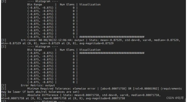

 

5. Practical operation: Use TensorRT to optimize the model

Set different quantization strategies for VGG

You can use PyTorch's quantization API and torch.quantizationmodules. PyTorch provides different quantization strategies and configuration options.

Sample code:

import torch
import torchvision
import torch.quantization

# Step 1: 加载VGG模型
model = torchvision.models.vgg16(pretrained=True)
model.eval()  # 将模型设置为评估模式

# Step 2: 定义量化配置
# 可以设置不同层的量化配置，例如设置量化位数、量化范围等
quant_config = torch.quantization.default_qconfig
quant_config_dict = {
    torch.nn.Conv2d: torch.quantization.default_qconfig,
    torch.nn.Linear: torch.quantization.default_qconfig
}

# Step 3: 量化感知训练
qat_model = torch.quantization.quantize_dynamic(model, quant_config_dict, dtype=torch.qint8)

# Step 4: 导出量化感知训练后的模型
torch.save(qat_model.state_dict(), "qat_vgg_model.pth")

5.2.2 Build a self-attention module and different versions of TRT to optimize attention

Code:

import torch
import torch.nn as nn
import tensorrt as trt
import numpy as np

# Step 1: 构建Self-Attention模块
class SelfAttention(nn.Module):
    def __init__(self, in_channels, key_channels, value_channels):
        super(SelfAttention, self).__init__()
        self.key_channels = key_channels
        self.value_channels = value_channels

        self.query = nn.Conv2d(in_channels, key_channels, kernel_size=1)
        self.key = nn.Conv2d(in_channels, key_channels, kernel_size=1)
        self.value = nn.Conv2d(in_channels, value_channels, kernel_size=1)

    def forward(self, x):
        query = self.query(x)
        key = self.key(x)
        value = self.value(x)

        attention_map = torch.matmul(query.view(query.size(0), self.key_channels, -1).permute(0, 2, 1),
                                     key.view(key.size(0), self.key_channels, -1))
        attention_map = nn.functional.softmax(attention_map, dim=-1)

        out = torch.matmul(attention_map, value.view(value.size(0), self.value_channels, -1))
        out = out.view(x.size(0), self.value_channels, *x.size()[2:])
        return out

# Step 2: 创建示例输入并导出模型为ONNX格式
model = SelfAttention(in_channels=64, key_channels=32, value_channels=32)
x = torch.randn(1, 64, 32, 32)
onnx_file = "self_attention.onnx"
torch.onnx.export(model, x, onnx_file, opset_version=11)

# Step 3: 使用TensorRT优化模型
TRT_LOGGER = trt.Logger(trt.Logger.WARNING)
with trt.Builder(TRT_LOGGER) as builder, builder.create_network() as network, trt.OnnxParser(network, TRT_LOGGER) as parser:
    with open(onnx_file, "rb") as model:
        parser.parse(model.read())
    builder.max_workspace_size = 1 << 30
    engine = builder.build_cuda_engine(network)

# Step 4: 保存优化后的模型
trt_file = "self_attention.trt"
with open(trt_file, "wb") as f:
    f.write(engine.serialize())

print("TensorRT engine created successfully and saved as:", trt_file)

Summarize:

        After studying the entire article, I believe you have mastered the entire development process of tensorrt. You can use different optimization solutions to improve the model in a targeted manner. If you need to expand your knowledge more deeply, please leave a message and communicate with each other. Thank you very much! ! ! !

PS: It is purely for learning and sharing experience, and does not participate in commercial value operations. If there is any infringement, please contact us in time! ! !

Preview of the next content:

• Deep learning model deployment OpenVINO acceleration