最近yolov5-7.0を徹底的に勉強していて、公式のコードが比較的読みやすいと感じているので、ネットワークの構造がよく理解できてきたのですが、その中でもアンカーボックスの生成の詳細がよくわかりませんを理解したいので先に進みました。前後のコードをよく見てください。それでは、学習の成果を記録していきます。個人的な意見ですので、ご不明な点がございましたらご指摘ください
1. アンカーフレームの仕組みを整理する
アンカー、アプリオリ ボックス、事前選択ボックスはすべて同じものです。つまり、入力データが特徴抽出段階を通過するとき、通常はダウンサンプリングが行われてデータ量を削減し、高レベルの特徴マップが取得されます。これらの高レベルの特徴マッププリセットのアンカー ボックスとラベル グランド トゥルースは損失計算に使用され、ネットワークのパラメータは勾配逆伝播に基づいて更新され、ネットワークのパラメータが位置とカテゴリを直接識別できるように徐々に反復されます。保存後、特定のタイプのターゲットを識別するためのネットワークのネットワーク重みファイルを取得します。
したがって、アンカー ボックスは通常、特徴抽出の最終段階で事前に設定されます。この段階では、低解像度の特徴マップが生成されます。yolov5s では、Detect の最後の層によって生成された 80 x 80、40 x 40、20 x 20 の特徴です。 . マップを作成し、特徴マップに基づいてアンカー ボックスをプリセットします。アンカーボックスに関しては、yolov5s.yamlに直接確認できる情報があります。
2. アンカーボックスはどのように機能しますか?
では、このアンカーボックスは具体的にどのように機能するのでしょうか? 特徴抽出の最終段階である Detect のコードを見てみましょう (models/yolo.py)
class Detect(nn.Module):
    # YOLOv5 Detect head for detection models
    stride = None  # strides computed during build
    dynamic = False  # force grid reconstruction
    export = False  # export mode

    def __init__(self, nc=80, anchors=(), ch=(), inplace=True):  # detection layer
        super().__init__()
        self.nc = nc  # number of classes
        self.no = nc + 5  # number of outputs per anchor
        self.nl = len(anchors)  # number of detection layers
        self.na = len(anchors[0]) // 2  # number of anchors
        self.grid = [torch.empty(0) for _ in range(self.nl)]  # init grid
        self.anchor_grid = [torch.empty(0) for _ in range(self.nl)]  # init anchor grid
        self.register_buffer('anchors', torch.tensor(anchors).float().view(self.nl, -1, 2))  # shape(nl,na,2)
        self.m = nn.ModuleList(nn.Conv2d(x, self.no * self.na, 1) for x in ch)  # output conv
        self.inplace = inplace  # use inplace ops (e.g. slice assignment)

    def forward(self, x):
        z = []  # inference output
        for i in range(self.nl):
            x[i] = self.m[i](x[i])  # conv
            bs, _, ny, nx = x[i].shape  # x(bs,255,20,20) to x(bs,3,20,20,85)
            x[i] = x[i].view(bs, self.na, self.no, ny, nx).permute(0, 1, 3, 4, 2).contiguous()

            if not self.training:  # inference
                if self.dynamic or self.grid[i].shape[2:4] != x[i].shape[2:4]:
                    self.grid[i], self.anchor_grid[i] = self._make_grid(nx, ny, i)

                if isinstance(self, Segment):  # (boxes + masks)
                    xy, wh, conf, mask = x[i].split((2, 2, self.nc + 1, self.no - self.nc - 5), 4)
                    xy = (xy.sigmoid() * 2 + self.grid[i]) * self.stride[i]  # xy
                    wh = (wh.sigmoid() * 2) ** 2 * self.anchor_grid[i]  # wh
                    y = torch.cat((xy, wh, conf.sigmoid(), mask), 4)
                else:  # Detect (boxes only)
                    xy, wh, conf = x[i].sigmoid().split((2, 2, self.nc + 1), 4)
                    xy = (xy * 2 + self.grid[i]) * self.stride[i]  # xy
                    wh = (wh * 2) ** 2 * self.anchor_grid[i]  # wh
                    y = torch.cat((xy, wh, conf), 4)
                z.append(y.view(bs, self.na * nx * ny, self.no))

        return x if self.training else (torch.cat(z, 1),) if self.export else (torch.cat(z, 1), x)

    def _make_grid(self, nx=20, ny=20, i=0, torch_1_10=check_version(torch.__version__, '1.10.0')):
        d = self.anchors[i].device
        t = self.anchors[i].dtype
        shape = 1, self.na, ny, nx, 2  # grid shape
        y, x = torch.arange(ny, device=d, dtype=t), torch.arange(nx, device=d, dtype=t)
        yv, xv = torch.meshgrid(y, x, indexing='ij') if torch_1_10 else torch.meshgrid(y, x)  # torch>=0.7 compatibility
        grid = torch.stack((xv, yv), 2).expand(shape) - 0.5  # add grid offset, i.e. y = 2.0 * x - 0.5
        anchor_grid = (self.anchors[i] * self.stride[i]).view((1, self.na, 1, 1, 2)).expand(shape)
        return grid, anchor_grid
Detect クラスにはアンカー パラメーター入力があり、アンカー情報がこのクラスで使用されていることを示していることがわかります。クラス内のアンカーに関連するコードの 1 つは次のとおりです。
self.register_buffer('anchors', torch.tensor(anchors).float().view(self.nl, -1, 2)) # shape(nl,na,2)
もう 1 つは、forward 関数の下にある _make_grid 関数です。ただし、forward 関数はトレーニング フェーズ中にこの関数を実行しないため、特徴マップ上でアンカー ボックスがどのように生成されるかを理解するのは困難です。
if not self.training:  # inference
    if self.dynamic or self.grid[i].shape[2:4] != x[i].shape[2:4]:
    	self.grid[i], self.anchor_grid[i] = self._make_grid(nx, ny, i)
次に、Detect クラスのトレーニング フェーズ中に実行されるコードは次のとおりです。
class Detect(nn.Module):
    # YOLOv5 Detect head for detection models
    stride = None  # strides computed during build
    dynamic = False  # force grid reconstruction
    export = False  # export mode

    def __init__(self, nc=80, anchors=(), ch=(), inplace=True):  # detection layer
        super().__init__()
        self.nc = nc  # number of classes
        self.no = nc + 5  # number of outputs per anchor
        self.nl = len(anchors)  # number of detection layers
        self.na = len(anchors[0]) // 2  # number of anchors
        self.grid = [torch.empty(0) for _ in range(self.nl)]  # init grid
        self.anchor_grid = [torch.empty(0) for _ in range(self.nl)]  # init anchor grid
        self.register_buffer('anchors', torch.tensor(anchors).float().view(self.nl, -1, 2))  # shape(nl,na,2)
        self.m = nn.ModuleList(nn.Conv2d(x, self.no * self.na, 1) for x in ch)  # output conv
        self.inplace = inplace  # use inplace ops (e.g. slice assignment)

    def forward(self, x):
        z = []  # inference output
        for i in range(self.nl):
            x[i] = self.m[i](x[i])  # conv
            bs, _, ny, nx = x[i].shape  # x(bs,255,20,20) to x(bs,3,20,20,85)
            x[i] = x[i].view(bs, self.na, self.no, ny, nx).permute(0, 1, 3, 4, 2).contiguous()

        return x if self.training else (torch.cat(z, 1),) if self.export else (torch.cat(z, 1), x)
これは、アンカーと密接に関係する唯一の register_buffer() 関数について言わなければなりません。以前、Detect クラスを含む BaseModel クラスと DetectionModel クラスを見ましたが、敷設を伴う操作は見つかりませんでした。アンカーボックス。
3. register_buffer() 関数
register_buffer() 関数はアンカーをパラメーターとしてネットワークに固定できることがわかり、この関数によって渡されるパラメーターはトレーニングの反復によって変化せず、出力はネットワーク トレーニングの最後にモデルとともに保存されます。register_buffer() 関数と register_parameter() 関数、nn.Parameter()、model.state_dict()、model.parameters()、および model.buffers() の関数と相違点を確認できます。Pytorch モデルで表示されるパラメーターとバッファー
デバッグ中に作成した記録は次のとおりです。
class Detect(nn.Module):
    # YOLOv5 Detect head for detection models
    stride = None  # strides computed during build
    dynamic = False  # force grid reconstruction
    export = False  # export mode

    def __init__(self, nc=80, anchors=(), ch=(), inplace=True):  # detection layer
        super().__init__()
        self.nc = nc  # number of classes
        self.no = nc + 5  # number of outputs per anchor
        self.nl = len(anchors)  # number of detection layers
        self.na = len(anchors[0]) // 2  # number of anchors
        self.grid = [torch.empty(0) for _ in range(self.nl)]  # init grid
        self.anchor_grid = [torch.empty(0) for _ in range(self.nl)]  # init anchor grid
        self.register_buffer('anchors', torch.tensor(anchors).float().view(self.nl, -1, 2))  # shape(nl,na,2)
        """anchors"""
        """ register_buffer的参数不参与梯度更新,最终随模型保存输出,此处把传入的anchors参数的数据通过register_buffer传入到网络中,"""
        """torch.tensor(anchors).float()
                tensor([[ 10.,  13.,  16.,  30.,  33.,  23.],
                        [ 30.,  61.,  62.,  45.,  59., 119.],
                        [116.,  90., 156., 198., 373., 326.]])
                ipdb> torch.tensor(anchors).float().view(self.nl, -1, 2)
                tensor([[[ 10.,  13.],
                        [ 16.,  30.],
                        [ 33.,  23.]],

                        [[ 30.,  61.],
                        [ 62.,  45.],
                        [ 59., 119.]],

                        [[116.,  90.],
                        [156., 198.],
                        [373., 326.]]])
                ipdb> self.anchor_grid
                [tensor([]), tensor([]), tensor([])]
                ipdb> anchors
                [[10, 13, 16, 30, 33, 23], [30, 61, 62, 45, 59, 119], [116, 90, 156, 198, 373, 326]]
                """
        # import ipdb;ipdb.set_trace()
        self.m = nn.ModuleList(nn.Conv2d(x, self.no * self.na, 1) for x in ch)  # output conv
        self.inplace = inplace  # use inplace ops (e.g. slice assignment)

        """ Detect层对输入的三个下采样倍数的数据分别采用三个全连接层输出
        self.m=
            ModuleList(
            (0): Conv2d(128, 18, kernel_size=(1, 1), stride=(1, 1))
            (1): Conv2d(256, 18, kernel_size=(1, 1), stride=(1, 1))
            (2): Conv2d(512, 18, kernel_size=(1, 1), stride=(1, 1))
            )
            其中输出维度 self.no * self.na,即此处的 18,表示每个维度三种尺度的锚框 x ( 类别 + xywh + score) = 3 x 6
        """

    def forward(self, x):
        """self.state_dict()
                anchors
                m.0.weight
                m.0.bias
                m.1.weight
                m.1.bias
                m.2.weight
                m.2.bias
        """

        """对应8,16,32倍下采样输出的特征图
            x:  x[0].shape
                torch.Size([1, 128, 32, 32])
                ipdb> x[1].shape
                torch.Size([1, 256, 16, 16])
                ipdb> x[2].shape
                torch.Size([1, 512, 8, 8])
        """
        z = []  # inference output
        import ipdb;ipdb.set_trace()
        for i in range(self.nl):
            x[i] = self.m[i](x[i])  # conv
            """经过全连接层后数据维度
            x[0].shape
                        = torch.Size([1, 18, 32, 32])
                x[1].shape
                        = torch.Size([1, 18, 16, 16])
                x[2].shape
                        = torch.Size([1, 18, 8, 8])
            """
            bs, _, ny, nx = x[i].shape  # x(bs,255,20,20) to x(bs,3,20,20,85)
            x[i] = x[i].view(bs, self.na, self.no, ny, nx).permute(0, 1, 3, 4, 2).contiguous()

            """训练阶段 对应8,16,32倍下采样输出的特征图在Detect类输出的数据维度
                x:x[0].shape
                        torch.Size([1, 3, 32, 32, 6])
                        ipdb> x[1].shape
                        torch.Size([1, 3, 16, 16, 6])
                        ipdb> x[2].shape
                        torch.Size([1, 3, 8, 8, 6])
            """

            if not self.training:  # inference
                if self.dynamic or self.grid[i].shape[2:4] != x[i].shape[2:4]:
                    self.grid[i], self.anchor_grid[i] = self._make_grid(nx, ny, i)

                if isinstance(self, Segment):  # (boxes + masks)
                    xy, wh, conf, mask = x[i].split((2, 2, self.nc + 1, self.no - self.nc - 5), 4)
                    xy = (xy.sigmoid() * 2 + self.grid[i]) * self.stride[i]  # xy
                    wh = (wh.sigmoid() * 2) ** 2 * self.anchor_grid[i]  # wh
                    y = torch.cat((xy, wh, conf.sigmoid(), mask), 4)
                else:  # Detect (boxes only)
                    xy, wh, conf = x[i].sigmoid().split((2, 2, self.nc + 1), 4)
                    """推断流程预测xywh"""
                    xy = (xy * 2 + self.grid[i]) * self.stride[i]  # xy
                    wh = (wh * 2) ** 2 * self.anchor_grid[i]  # wh
                    y = torch.cat((xy, wh, conf), 4)
                z.append(y.view(bs, self.na * nx * ny, self.no))

        return x if self.training else (torch.cat(z, 1),) if self.export else (torch.cat(z, 1), x)

    def _make_grid(self, nx=20, ny=20, i=0, torch_1_10=check_version(torch.__version__, '1.10.0')):
        d = self.anchors[i].device
        t = self.anchors[i].dtype
        shape = 1, self.na, ny, nx, 2  # grid shape
        y, x = torch.arange(ny, device=d, dtype=t), torch.arange(nx, device=d, dtype=t)
        yv, xv = torch.meshgrid(y, x, indexing='ij') if torch_1_10 else torch.meshgrid(y, x)  # torch>=0.7 compatibility
        grid = torch.stack((xv, yv), 2).expand(shape) - 0.5  # add grid offset, i.e. y = 2.0 * x - 0.5
        anchor_grid = (self.anchors[i] * self.stride[i]).view((1, self.na, 1, 1, 2)).expand(shape)
        return grid, anchor_grid
上記のデバッグ状況は、アンカー ボックスがパラメータを通じてネットワークに登録されていることも完全に示すことができます。forward() 関数では、Detect クラス構造のパラメータ状況である self を調べました。その中には self.state_dict() があります。 ----- -> アンカー、m.0.weight、m.0.bias、m.1.weight、m.1.bias、m.2.weight、m.2.bias にはアンカーが含まれます。
4. アンカーボックスの具体的な生成
アンカー ボックスの具体的な生成は次のようになります。
def forward(self, x):
"""输入x是进入Detect的三个尺度的特征图"""
        z = []  # inference output
        for i in range(self.nl):
        """self.nl=3表示Detect对应三个尺度用以处理三层特征图的网络结构,
        	self.m是对应三个尺度特征图的网络结构,对应不同的输入数据维度,输出维度都是18,其中输出维度 self.no * self.na,即此处的 18,表示每个维度三种尺度的锚框 x ( 类别 + xywh + score) = 3 x 6
        	self.m=
            ModuleList(
            (0): Conv2d(128, 18, kernel_size=(1, 1), stride=(1, 1))
            (1): Conv2d(256, 18, kernel_size=(1, 1), stride=(1, 1))
            (2): Conv2d(512, 18, kernel_size=(1, 1), stride=(1, 1))
            )"""
            x[i] = self.m[i](x[i])  # conv
            """对应的输入特征图在对应的m的网络结构中进行计算
            	x[0].shape
                        = torch.Size([1, 18, 32, 32])
                x[0].shape
                        = torch.Size([1, 18, 16, 16])
                x[2].shape
                        = torch.Size([1, 18, 8, 8])"""
            bs, _, ny, nx = x[i].shape  # x(bs,255,20,20) to x(bs,3,20,20,85)
            x[i] = x[i].view(bs, self.na, self.no, ny, nx).permute(0, 1, 3, 4, 2).contiguous()
            """改变数据输出维度便于后续处理
            	x:x[0].shape
                        torch.Size([1, 3, 32, 32, 6])
                        ipdb> x[1].shape
                        torch.Size([1, 3, 16, 16, 6])
                        ipdb> x[2].shape
                        torch.Size([1, 3, 8, 8, 6])
                 维度变换:1表示batch_size;3表示3种尺度的锚框;32,32表示特征图维度;6表示预测结果,含类别 + x、y、w、h + score
            """
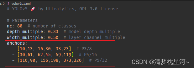
yolov5s.yamlのアンカー情報を見てください。
anchors:
  - [10,13, 16,30, 33,23]  # P3/8
  - [30,61, 62,45, 59,119]  # P4/16
  - [116,90, 156,198, 373,326]  # P5/32
このうち、10、13、16、30、33、23 はそれぞれアンカー ボックスの 3 つのプリセット スケールを表し、アンカー ボックスの幅と高さを示します。他の 2 行は同じで、8 倍、16 倍に対応しますサンプリング倍数の出力特徴マップのアンカー ボックスがプリセットされているため、各スケールの出力特徴マップは 3 つのスケールのアンカー ボックスの出力特徴マップを生成し、3 つのスケールの特徴マップは、合計 9 つのスケールのアンカー ボックスを生成します。
したがって、Detect クラスを介して特徴マップに基づいてデータが予測されており、特徴マップ データにプリセット アンカーを掛け合わせたものであるため、説明ネットワークによってはターゲット位置のオフセットを予測していることがわかります。ボックス パラメーターはターゲットの位置を取得しますが、ターゲットの位置を直接予測するものではありません。
このうち、データのアンカーボックス情報を取得する場合、
実際にデータ情報はBaseModelクラスの_forward_once関数内で処理されます。
class DetectionModel(BaseModel):
	......
	def forward(self, x, augment=False, profile=False, visualize=False):
        if augment:
            return self._forward_augment(x)  # augmented inference, None
        return self._forward_once(x, profile, visualize)  # single-scale inference, train

class BaseModel(nn.Module):
    # YOLOv5 base model
    def forward(self, x, profile=False, visualize=False):
        return self._forward_once(x, profile, visualize)  # single-scale inference, train

    def _forward_once(self, x, profile=False, visualize=False):
        y, dt = [], []  # outputs
        for m in self.model:
        """self.model是构建好的网络结构,输入x是实际数据"""
            if m.f != -1:  # if not from previous layer
                x = y[m.f] if isinstance(m.f, int) else [x if j == -1 else y[j] for j in m.f]  # from earlier layers
            if profile:
                self._profile_one_layer(m, x, dt)
            x = m(x)  # run
            y.append(x if m.i in self.save else None)  # save output
            if visualize:
                feature_visualization(x, m.type, m.i, save_dir=visualize)
        return x
        .......
ここでの x 出力は、train.py の pred 出力と同等です。
with torch.cuda.amp.autocast(amp):
    pred = model(imgs)  # forward
    loss, loss_items = compute_loss(pred, targets.to(device))  # loss scaled by batch_size```
アンカーボックスを可視化したい場合はpredの処理を推奨、具体的な処理方法についてはDetectクラスの未学習のコードを参照することを推奨します。
事前トレーニング済みモデルが使用される場合、事前トレーニング済みモデルは一定量のデータでトレーニングされており、ネットワーク パラメーターにはターゲットに対する特定の認識能力があるため、アンカー ボックスの表示効果は良好ではない可能性があります。
5. まとめ
yolov5s では、アンカーは、プリセットされたアンカー ボックスのスケール情報をパラメータとして register_buffer() 関数を通じて最終的な検出ネットワーク層に登録します。ターゲットの位置情報は、アンカー ボックスのパラメータと特徴マップ データを乗算することによって得られるため、ネットワークはアンカー ボックスに対する相対的な位置情報を予測し、これはアンカー ボックスの位置オフセットとして理解できます。ターゲットの位置オフセットは、ターゲット カテゴリの識別と位置予測を実現するために使用されます。