MobileNet v1 ネットワーク
MobileNet ネットワークは、モバイルまたは組み込みデバイスの軽量 CNN ネットワークに焦点を当てています。従来の畳み込みニューラルネットワークと比較して、精度の若干の低下を前提としてモデルパラメータと計算量が大幅に削減されます。VGG16と比較すると正解率は0.9%低下しますが、モデルパラメータはVGGの1/32にとどまります
1.Depthwise Convolution(計算量とパラメータ数を大幅に削減)
2.ハイパーパラメータα、βの増加。
MobileNet v1 ネットワークと比較して
、MobileNet v2 ネットワークは精度が高く、モデルが小型です。
1.Inverted Residuals (反転残差構造)
2.線形ボトルネック
MovileNet v3 ネットワーク
1. ブロックの更新 (ネック、SE モジュールの追加、アクティベーション機能の更新)
2. NAS 検索パラメーターの使用 (ニューラル アーキテクチャ検索)
3. 時間のかかるレイヤー構造の再設計
ShuffleNet v1 ネットワーク
1. チャネル シャッフルのアイデアを提案
2. ShuffleNet ユニットは GConv と DWConv でいっぱい
論文「HybridSN: ハイパースペクトル画像分類のための 3-D–2-DCNN 特徴階層の探索」を読んで、3D 畳み込みと 2D 畳み込みの違いについて考えてください。
コードを Colab に入力して実行します。ネットワーク部分は自分で完了する必要があります。
#Spectral Python (SPy)是一个用于处理高光谱图像数据的纯Python模块。
#它具有读取、显示、操作和分类高光谱图像的功能。之所以用它是因为这个对多波段图像的支持更好
! pip install spectral
#导入所使用的库
import numpy as np
import matplotlib.pyplot as plt
import scipy.io as sio
from sklearn.decomposition import PCA
from sklearn.model_selection import train_test_split
from sklearn.metrics import confusion_matrix, accuracy_score, classification_report, cohen_kappa_score
import spectral
import torch
import torchvision
import torch.nn as nn
import torch.nn.functional as F
import torch.optim as optim
#导入云盘中上传的文件
from google.colab import drive
drive.mount('/content/drive/')
import scipy.io as sio
import os
filepath = os.path.join('/content/drive/My Drive/Deeplearning/Indian_pines_corrected.mat')
filepath1 = os.path.join('/content/drive/My Drive/Deeplearning/Indian_pines_gt.mat')
#定义HybridSN类
class_num = 16
class HybridSN(nn.Module):
  def __init__(self,num_classes=16):
    super(HybridSN,self).__init__()
    self.conv1 = nn.Conv3d(1,8,(7,3,3))
    self.bn1=nn.BatchNorm3d(8)

    self.conv2 = nn.Conv3d(8,16,(5,3,3))
    self.bn2=nn.BatchNorm3d(16)

    self.conv3 = nn.Conv3d(16,32,(3,3,3))
    self.bn3=nn.BatchNorm3d(32)

    self.conv4 = nn.Conv2d(576,64,(3,3))
    self.bn4=nn.BatchNorm2d(64)

    self.drop = nn.Dropout(p=0.4)

    self.fc1 = nn.Linear(18496,256)
    self.fc2 = nn.Linear(256,128)
    self.fc3 = nn.Linear(128,num_classes)

    self.relu = nn.ReLU()

    self.softmax = nn.Softmax(dim=1)

  def forward(self,x):
    out = self.relu(self.bn1(self.conv1(x)))
    out = self.relu(self.bn2(self.conv2(out)))
    out = self.relu(self.bn3(self.conv3(out)))

    out = out.view(-1,out.shape[1]*out.shape[2],out.shape[3],out.shape[4])
    out = self.relu(self.bn4(self.conv4(out)))

    out = out.view(out.size(0),-1)
    out = self.fc1(out)
    out = self.drop(out)
    out = self.relu(out)
    out = self.fc2(out)
    out = self.drop(out)
    out = self.relu(out)
    out = self.fc3(out)
    # out = self.softmax(out)
    return out


# 随机输入,测试网络结构是否通
x = torch.randn(1,1,30,25,25)
net = HybridSN()
y = net(x)
print(y.shape)
# 创建数据集
# 对高光谱数据 X 应用 PCA 变换
def applyPCA(X, numComponents):
    newX = np.reshape(X, (-1, X.shape[2]))
    pca = PCA(n_components=numComponents, whiten=True)
    newX = pca.fit_transform(newX)
    newX = np.reshape(newX, (X.shape[0], X.shape[1], numComponents))
    return newX

# 对单个像素周围提取 patch 时,边缘像素就无法取了,因此,给这部分像素进行 padding 操作
def padWithZeros(X, margin=2):
    newX = np.zeros((X.shape[0] + 2 * margin, X.shape[1] + 2* margin, X.shape[2]))
    x_offset = margin
    y_offset = margin
    newX[x_offset:X.shape[0] + x_offset, y_offset:X.shape[1] + y_offset, :] = X
    return newX

# 在每个像素周围提取 patch ,然后创建成符合 keras 处理的格式
def createImageCubes(X, y, windowSize=5, removeZeroLabels = True):
    # 给 X 做 padding
    margin = int((windowSize - 1) / 2)
    zeroPaddedX = padWithZeros(X, margin=margin)
    # split patches
    patchesData = np.zeros((X.shape[0] * X.shape[1], windowSize, windowSize, X.shape[2]))
    patchesLabels = np.zeros((X.shape[0] * X.shape[1]))
    patchIndex = 0
    for r in range(margin, zeroPaddedX.shape[0] - margin):
        for c in range(margin, zeroPaddedX.shape[1] - margin):
            patch = zeroPaddedX[r - margin:r + margin + 1, c - margin:c + margin + 1]
            patchesData[patchIndex, :, :, :] = patch
            patchesLabels[patchIndex] = y[r-margin, c-margin]
            patchIndex = patchIndex + 1
    if removeZeroLabels:
        patchesData = patchesData[patchesLabels>0,:,:,:]
        patchesLabels = patchesLabels[patchesLabels>0]
        patchesLabels -= 1
    return patchesData, patchesLabels

def splitTrainTestSet(X, y, testRatio, randomState=345):
    X_train, X_test, y_train, y_test = train_test_split(X, y, test_size=testRatio, random_state=randomState, stratify=y)
    return X_train, X_test, y_train, y_test
#读取并创建数据集
# 地物类别
class_num = 16
X = sio.loadmat(filepath)['indian_pines_corrected']
y = sio.loadmat(filepath1)['indian_pines_gt']
# 用于测试样本的比例
test_ratio = 0.90
# 每个像素周围提取 patch 的尺寸
patch_size = 25
# 使用 PCA 降维,得到主成分的数量
pca_components = 30
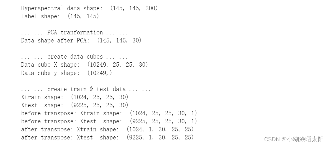
print('Hyperspectral data shape: ', X.shape)
print('Label shape: ', y.shape)
print('\n... ... PCA tranformation ... ...')
X_pca = applyPCA(X, numComponents=pca_components)
print('Data shape after PCA: ', X_pca.shape)
print('\n... ... create data cubes ... ...')
X_pca, y = createImageCubes(X_pca, y, windowSize=patch_size)
print('Data cube X shape: ', X_pca.shape)
print('Data cube y shape: ', y.shape)
print('\n... ... create train & test data ... ...')
Xtrain, Xtest, ytrain, ytest = splitTrainTestSet(X_pca, y, test_ratio)
print('Xtrain shape: ', Xtrain.shape)
print('Xtest shape: ', Xtest.shape)
# 改变 Xtrain, Ytrain 的形状,以符合 keras 的要求
Xtrain = Xtrain.reshape(-1, patch_size, patch_size, pca_components, 1)
Xtest = Xtest.reshape(-1, patch_size, patch_size, pca_components, 1)
print('before transpose: Xtrain shape: ', Xtrain.shape)
print('before transpose: Xtest shape: ', Xtest.shape)
# 为了适应 pytorch 结构,数据要做 transpose
Xtrain = Xtrain.transpose(0, 4, 3, 1, 2)
Xtest = Xtest.transpose(0, 4, 3, 1, 2)
print('after transpose: Xtrain shape: ', Xtrain.shape)
print('after transpose: Xtest shape: ', Xtest.shape)
""" Training dataset"""
class TrainDS(torch.utils.data.Dataset):
def __init__(self):
self.len = Xtrain.shape[0]
self.x_data = torch.FloatTensor(Xtrain)
self.y_data = torch.LongTensor(ytrain)
def __getitem__(self, index):
# 根据索引返回数据和对应的标签
return self.x_data[index], self.y_data[index]
def __len__(self):
# 返回文件数据的数目
return self.len
""" Testing dataset"""
class TestDS(torch.utils.data.Dataset):
def __init__(self):
self.len = Xtest.shape[0]
self.x_data = torch.FloatTensor(Xtest)
self.y_data = torch.LongTensor(ytest)
def __getitem__(self, index):
# 根据索引返回数据和对应的标签
return self.x_data[index], self.y_data[index]
def __len__(self):
# 返回文件数据的数目
return self.len
# 创建 trainloader 和 testloader
trainset = TrainDS()
testset = TestDS()
train_loader = torch.utils.data.DataLoader(dataset=trainset, batch_size=128, shuffle=True, num_workers=2)
test_loader = torch.utils.data.DataLoader(dataset=testset, batch_size=128, shuffle=False, num_workers=2)
# 使用GPU训练,可以在菜单 "代码执行工具" -> "更改运行时类型" 里进行设置
device = torch.device("cuda:0" if torch.cuda.is_available() else "cpu")
# 网络放到GPU上
net = HybridSN().to(device)
criterion = nn.CrossEntropyLoss()
optimizer = optim.Adam(net.parameters(), lr=0.001)
# 开始训练
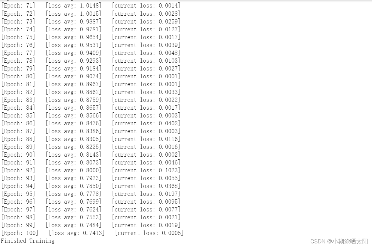
total_loss = 0
for epoch in range(100):
for i, (inputs, labels) in enumerate(train_loader):
inputs = inputs.to(device)
labels = labels.to(device)
# 优化器梯度归零
optimizer.zero_grad()
# 正向传播 + 反向传播 + 优化
outputs = net(inputs)
loss = criterion(outputs, labels)
loss.backward()
optimizer.step()
total_loss += loss.item()
print('[Epoch: %d] [loss avg: %.4f] [current loss: %.4f]' %(epoch + 1, total_loss/(epoch+1), loss.item()))
print('Finished Training')
#模型测试
count = 0
# 模型测试
for inputs, _ in test_loader:
inputs = inputs.to(device)
outputs = net(inputs)
outputs = np.argmax(outputs.detach().cpu().numpy(), axis=1)
if count == 0:
y_pred_test = outputs
count = 1
else:
y_pred_test = np.concatenate( (y_pred_test, outputs) )
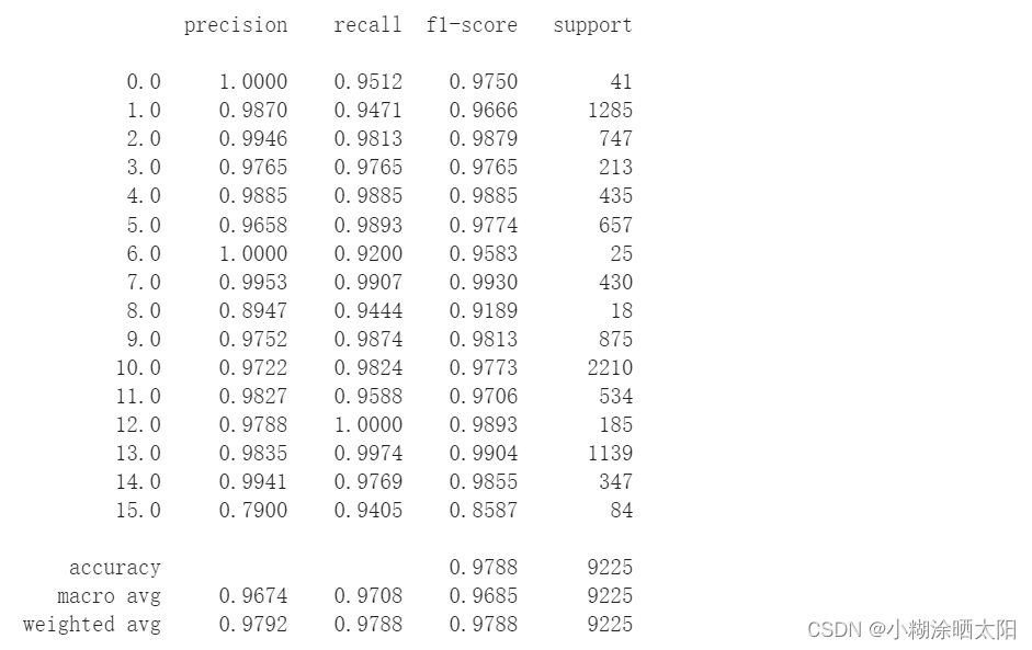
# 生成分类报告
classification = classification_report(ytest, y_pred_test, digits=4)
print(classification)
#备用函数,用于计算各个类准确率
from operator import truediv

def AA_andEachClassAccuracy(confusion_matrix):
    counter = confusion_matrix.shape[0]
    list_diag = np.diag(confusion_matrix)
    list_raw_sum = np.sum(confusion_matrix, axis=1)
    each_acc = np.nan_to_num(truediv(list_diag, list_raw_sum))
    average_acc = np.mean(each_acc)
    return each_acc, average_acc


def reports (test_loader, y_test, name):
    count = 0
    # 模型测试
    for inputs, _ in test_loader:
        inputs = inputs.to(device)
        outputs = net(inputs)
        outputs = np.argmax(outputs.detach().cpu().numpy(), axis=1)
        if count == 0:
            y_pred =  outputs
            count = 1
        else:
            y_pred = np.concatenate( (y_pred, outputs) )

    if name == 'IP':
        target_names = ['Alfalfa', 'Corn-notill', 'Corn-mintill', 'Corn'
                        ,'Grass-pasture', 'Grass-trees', 'Grass-pasture-mowed',
                        'Hay-windrowed', 'Oats', 'Soybean-notill', 'Soybean-mintill',
                        'Soybean-clean', 'Wheat', 'Woods', 'Buildings-Grass-Trees-Drives',
                        'Stone-Steel-Towers']
    elif name == 'SA':
        target_names = ['Brocoli_green_weeds_1','Brocoli_green_weeds_2','Fallow','Fallow_rough_plow','Fallow_smooth',
                        'Stubble','Celery','Grapes_untrained','Soil_vinyard_develop','Corn_senesced_green_weeds',
                        'Lettuce_romaine_4wk','Lettuce_romaine_5wk','Lettuce_romaine_6wk','Lettuce_romaine_7wk',
                        'Vinyard_untrained','Vinyard_vertical_trellis']
    elif name == 'PU':
        target_names = ['Asphalt','Meadows','Gravel','Trees', 'Painted metal sheets','Bare Soil','Bitumen',
                        'Self-Blocking Bricks','Shadows']

    classification = classification_report(y_test, y_pred, target_names=target_names)
    oa = accuracy_score(y_test, y_pred)
    confusion = confusion_matrix(y_test, y_pred)
    each_acc, aa = AA_andEachClassAccuracy(confusion)
    kappa = cohen_kappa_score(y_test, y_pred)

    return classification, confusion, oa*100, each_acc*100, aa*100, kappa*100
classification, confusion, oa, each_acc, aa, kappa = reports(test_loader, ytest, 'IP')
classification = str(classification)
confusion = str(confusion)
file_name = "classification_report.txt"

with open(file_name, 'w') as x_file:
    x_file.write('\n')
    x_file.write('{} Kappa accuracy (%)'.format(kappa))
    x_file.write('\n')
    x_file.write('{} Overall accuracy (%)'.format(oa))
    x_file.write('\n')
    x_file.write('{} Average accuracy (%)'.format(aa))
    x_file.write('\n')
    x_file.write('\n')
    x_file.write('{}'.format(classification))
    x_file.write('\n')
    x_file.write('{}'.format(confusion))
# load the original image
X = sio.loadmat(filepath)['indian_pines_corrected']
y = sio.loadmat(filepath1)['indian_pines_gt']
height = y.shape[0]
width = y.shape[1]
X = applyPCA(X, numComponents= pca_components)
X = padWithZeros(X, patch_size//2)
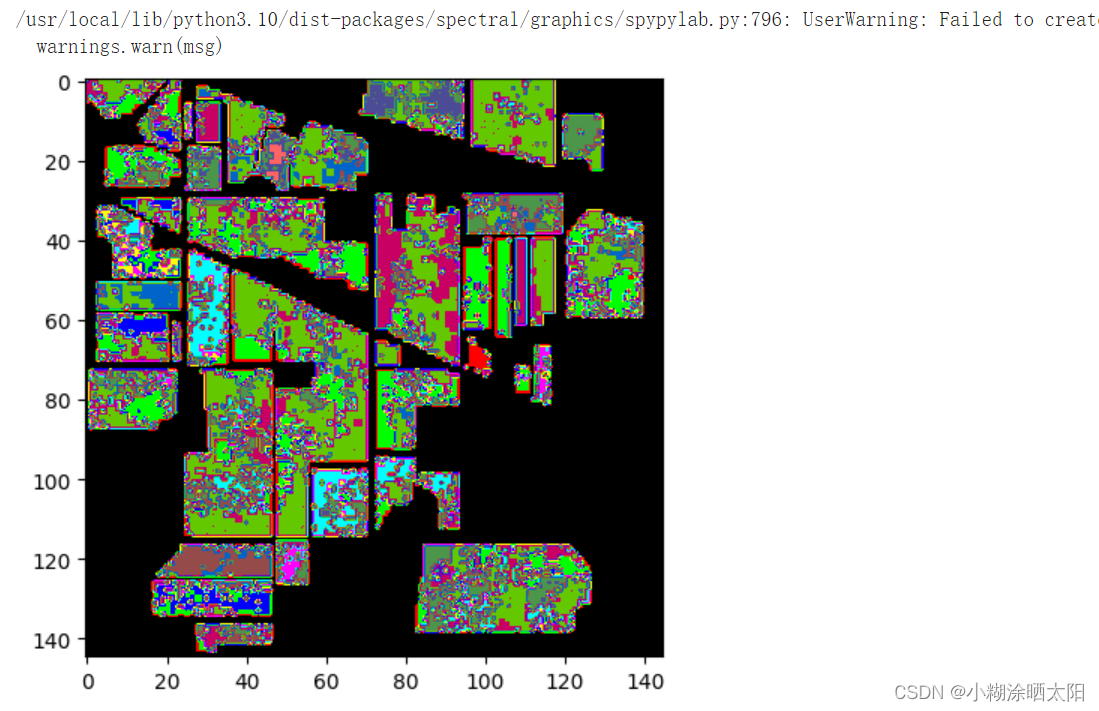
# 逐像素预测类别
outputs = np.zeros((height,width))
for i in range(height):
for j in range(width):
if int(y[i,j]) == 0:
continue
else :
image_patch = X[i:i+patch_size, j:j+patch_size, :]
image_patch = image_patch.reshape(1,image_patch.shape[0],image_patch.shape[1], image_patch.shape[2], 1)
X_test_image = torch.FloatTensor(image_patch.transpose(0, 4, 3, 1, 2)).to(device)
prediction = net(X_test_image)
prediction = np.argmax(prediction.detach().cpu().numpy(), axis=1)
outputs[i][j] = prediction+1
if i % 20 == 0:
print('... ... row ', i, ' handling ... ...')
predict_image = spectral.imshow(classes = outputs.astype(int),figsize =(5,5))
● HybridSN をトレーニングし、数回テストすると、各分類の結果が異なることがわかります。その理由を考えてください。
在进行训练时会采用梯度下降的方法,这些方法可能会找到局部最优解,但是因为你的学习率也就是你的步长设置的不够大,
就会导致模型被困在局部最优解,无法跳出。 其次,你每次训练的时候,神经网络的参数和权重每次都是随机的,所以肯定每次的结果都不一样。
● ハイパースペクトル画像の分類パフォーマンスをさらに向上させたい場合、どうすれば向上できますか?
1.增加大量、可靠的训练样本,提高泛化性能。
2.选择合适的网络结构。
3.确定超参数:在训练过程中,检验模型的状态、收敛情况。通常用来调整超参数,通过几组模型在验证集上的表现确定超参数。
4.对特征图每个位置进行二维调整(即attention调整),使模型关注到值得更多关注的区域上。
● 深さ方向の畳み込みとグループ畳み込みの違いと関係は何ですか?
分组卷积只进行一次卷积操作即可,而深度可分离卷积需要进行两次——先depth_wise再point_wise卷积,但他们本质上是一样的。
深度可分离卷积进行一次卷积是无法达到输出指定维度的tensor的,这是由它将group设为in_channel决定的,输出的tensor通道数只能是in_channel,不能达到要求,
所以又用了1*1的卷积改变最终输出的通道数。这样的想法也是自然而然的,BottleNeck不就是先1*1卷积减少参数量再3*3卷积feature map,最后再1*1恢复原来的通道数,
所以BottleNeck的目的就是减少参数量。提到BottleNeck结构就是想说明1*1卷积经常用来改变通道数。
● SENet の注意を空間位置に追加できますか?
● ShuffleNet では、コードでチャネル シャッフルを実装するにはどうすればよいですか?
def channel_shuffle(x: Tensor, groups: int) -> Tensor:

    batch_size, num_channels, height, width = x.size()
    channels_per_group = num_channels // groups

    # reshape
    # [batch_size, num_channels, height, width] -> [batch_size, groups, channels_per_group, height, width]
    x = x.view(batch_size, groups, channels_per_group, height, width)

    x = torch.transpose(x, 1, 2).contiguous()

    # flatten
    x = x.view(batch_size, -1, height, width)

    return x