ビジョン トランスフォーマーをゼロから構築する (Pytorch バージョン)

その他のコンテンツについては、公式アカウント「無敵の張道」をフォローしてください。

序文

2020 年に Dosovitskiy らによってビジョン トランスフォーマー (ViT) が提案された後、コンピューター ビジョンの分野で支配的な地位を徐々に占め、画像分類、ターゲット検出、セマンティック セグメンテーションなどのダウンストリーム タスクで優れたパフォーマンスを達成しています。 、CVフィールド波でトランスシリーズをオフにします。ここでは、ゼロから Pytorch フレームワークに基づいて ViT モデルを段階的に実装する方法を紹介します。

序文

自然言語処理 (NLP) で使用される Transformer モデルに慣れていない場合は、CV 分野での Transformer の適用について少し戸惑うかもしれませんし、画像での ViT モデルの使用についても明確ではありません。心配しないでください。最初から始める方法は次のとおりです。 (PyTorch を使用して) 私の最初の ViT を実装します。

タスクを定義する

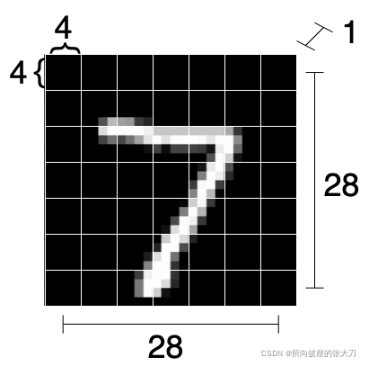
初心者向けに、画像分類用の MNIST 手書きデータセットであるエントリ データセットを選択します. 目標は単純ですが、この画像分類タスクに基づいて ViT モデルの全体的なコンテキストを明確にすることができます. MNISTデータセットを簡単に紹介すると、これは手書きの数字（[0–9]）のデータセットであり、画像はすべて28x28サイズのグレースケール画像です。
まず、使用する必要がある pytorch のいくつかのモジュールをインポートします。

import numpy as np
import torch
import torch.nn as nn
from torch.nn import CrossEntropyLoss
from torch.optim import Adam
from torch.utils.data import DataLoader
from torchvision.datasets.mnist import MNIST
from torchvision.transforms import ToTensor

MNIST データセットを前処理し、モデルをインスタンス化し、損失を定義し、Adam オプティマイザーを使用し、50 エポックのトレーニングを行い、テスト セットの精度を計算するメイン関数を作成しましょう。

def main():
    # Loading data
    transform = ToTensor()

    train_set = MNIST(root='./../datasets', train=True, download=True, transform=transform)
    test_set = MNIST(root='./../datasets', train=False, download=True, transform=transform)

    train_loader = DataLoader(train_set, shuffle=True, batch_size=16)
    test_loader = DataLoader(test_set, shuffle=False, batch_size=16)

    # Defining model and training options
    model = MyViT((1, 28, 28), n_patches=7, hidden_d=20, n_heads=2, out_d=10) # TODO define ViT model 
    N_EPOCHS = 50
    LR = 0.01

    # Training loop
    optimizer = Adam(model.parameters(), lr=LR)
    criterion = CrossEntropyLoss()
    for epoch in range(N_EPOCHS):
        train_loss = 0.0
        for batch in train_loader:
            x, y = batch
            y_hat = model(x)
            loss = criterion(y_hat, y) / len(x)

            train_loss += loss.item()

            optimizer.zero_grad()
            loss.backward()
            optimizer.step()

        print(f"Epoch {
      
      epoch + 1}/{
      
      N_EPOCHS} loss: {
      
      train_loss:.2f}")

 # Test loop
    correct, total = 0, 0
    test_loss = 0.0
    for batch in test_loader:
        x, y = batch
        y_hat = model(x)
        loss = criterion(y_hat, y) / len(x)
        test_loss += loss

        correct += torch.sum(torch.argmax(y_hat, dim=1) == y).item()
        total += len(x)
    print(f"Test loss: {
      
      test_loss:.2f}")
    print(f"Test accuracy: {
      
      correct / total * 100:.2f}%")

トレーニングとテストのフレームワーク全体を構築したら, ViT モデルの構築に取り掛かりましょう. モデルのタスクは (Nx1x28x28) 画像を分類することです. 最初に空の nn.Module クラスを定義し、徐々に埋めていきます:

class MyViT(nn.Module):
    def __init__(self):
        # Super constructor
        super(MyViT, self).__init__()

    def forward(self, images):
        pass

ViT アーキテクチャ

pytorch とほとんどの DL フレームワークは autograd 計算を提供するため、ViT モデルのフォワード パス プロセスだけを気にする必要があります.モデルのオプティマイザはトレーニング フレームワークで定義されており、pytorch フレームワークは勾配とモデルのパラメーターをトレーニングします。

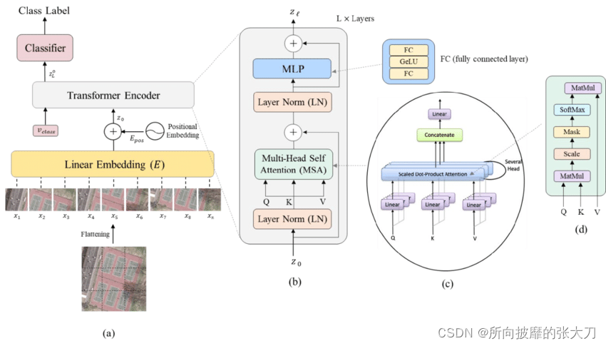
上の図は ViT のモデル ネットワーク アーキテクチャ全体を示しており、入力画像 (a) が最初に同じサイズのパッチ サブピクチャにカットされ、次に各サブピクチャが Linear Embedding に入れられることがわかります。画像ベクトル 完全な接続操作を行い、トランス入力の前処理を行い、なぜこの線形埋め込みを追加するのか、ここで [1] の著者の解釈を参照できます。著者はトランスシリーズについて非常に詳細に話しました。壁のひび。Linear Embedding 層を出た後、画像内の各パッチの相対的な位置情報を考慮するために Positonal エンコーディングを追加し、続いてトランスフォーマー エンコーダーの処理を行い、MLP の分類ヘッドを追加して画像の分類を出力します。 .

上の図は、[1] の著者が全員の理解を容易にするためのもので、進行プロセスにさまざまな側面を追加しています。以下では、6 つの主要なステップを経て ViT を構築します。

パッチ適用と線形マップ

Transformer エンコーダは、最初は主に NLP などのシリアル化されたデータに使用されました. CV フィールドで使用する最初のステップは、「シリアル化された」画像を処理することです. ここでの処理方法は、画像を複数のサブ画像に分解することです.各サブイメージをベクトルに変換します。
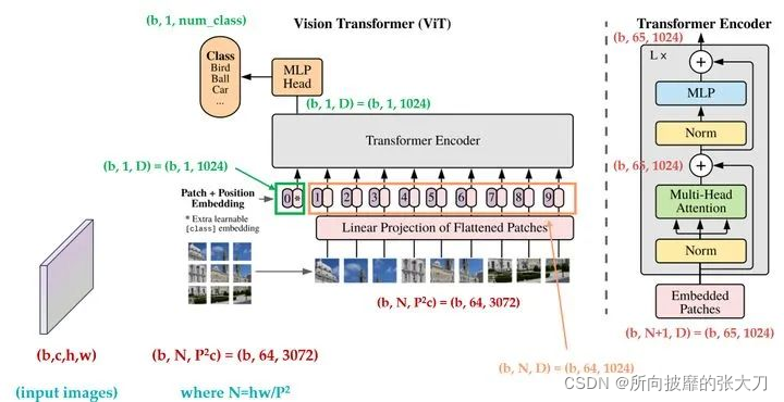
MNIST データセットでは、各 (1x28x28) 画像を 7x7 ブロックに分割します。各ブロック サイズは 4x4 です (ブロックが完全に分割できない場合、画像パディングを埋める必要があります)。単一の画像。元のグラフを次のように変形します:
(N, PxP, HxC/P x WxC/P) = (N, 7x7, 4x4) = (N, 49, 16)
各サブグラフのサイズは 1x4x4 ですが、平坦化して16 次元のベクトル。また、MNIST には 1 つのカラー チャネルしかありません。複数のカラー チャネルがある場合は、それらもベクトルにフラット化されます。

コードに上記の関数を実装します。

class MyViT(nn.Module):
    def __init__(self, input_shape, n_patches=7):
        # Super constructor
        super(MyViT, self).__init__()

        # Input and patches sizes
        self.input_shape = input_shape
        self.n_patches = n_patches
        assert input_shape[1] % n_patches == 0, "Input shape not entirely divisible by number of patches"
        assert input_shape[2] % n_patches == 0, "Input shape not entirely divisible by number of patches"


    def forward(self, images):
        # Dividing images into patches
        n, c, w, h = images.shape
        patches = images.reshape(n, self.n_patches ** 2, self.input_d)
        return patches 

フラット化されたパッチ (ベクトル) を取得し、任意のベクトル サイズにマップできる線形マップを介して次元を変更したので、「隠し次元」のクラス コンストラクターに hidden_​​d パラメーターを追加します。ここでは、隠れ次元が 8 であるため、16 次元の各パッチを 8 次元のパッチにマッピングします。実装コードは次のとおりです。

class MyViT(nn.Module):
    def __init__(self, input_shape, n_patches=7, hidden_d=8):
        # Super constructor
        super(MyViT, self).__init__()

        # Input and patches sizes
        self.input_shape = input_shape
        self.n_patches = n_patches
        assert input_shape[1] % n_patches == 0, "Input shape not entirely divisible by number of patches"
        assert input_shape[2] % n_patches == 0, "Input shape not entirely divisible by number of patches"
        self.hidden_d = hidden_d

        # 1) Linear mapper
        self.input_d = int(input_shape[0] * self.patch_size[0] * self.patch_size[1])
        self.linear_mapper = nn.Linear(self.input_d, self.hidden_d)

    def forward(self, images):
        # Dividing images into patches
        n, c, w, h = images.shape
        patches = images.reshape(n, self.n_patches ** 2, self.input_d)
         # Running linear layer for tokenization
        tokens = self.linear_mapper(patches)

        return tokens  

カテゴリ タグを追加する

隠れ層を追加した後, 分類タスクを完了するために, 分類マークを追加する必要があります. 主な理由は [1] を参照するためです. ここでは実装のみを行います. これで、(N, 49, 8) テンソルを (N, 50, 8) テンソルに変換するモデルにパラメーターを追加できます (各シーケンスに特別なマーカーを追加します)。

class MyViT(nn.Module):
    def __init__(self, input_shape, n_patches=7, hidden_d=8, n_heads=2, out_d=10):
        # Super constructor
        super(MyViT, self).__init__()

        # Input and patches sizes
        self.input_shape = input_shape
        self.n_patches = n_patches
        self.n_heads = n_heads
        assert input_shape[1] % n_patches == 0, "Input shape not entirely divisible by number of patches"
        assert input_shape[2] % n_patches == 0, "Input shape not entirely divisible by number of patches"
        self.hidden_d = hidden_d

        # 1) Linear mapper
        self.input_d = int(input_shape[0] * self.patch_size[0] * self.patch_size[1])
        self.linear_mapper = nn.Linear(self.input_d, self.hidden_d)

        # 2) Classification token
        self.class_token = nn.Parameter(torch.rand(1, self.hidden_d))

    def forward(self, images):
        # Dividing images into patches
        n, c, w, h = images.shape
        patches = images.reshape(n, self.n_patches ** 2, self.input_d)
         # Running linear layer for tokenization
        tokens = self.linear_mapper(patches)
        # Adding classification token to the tokens
        tokens = torch.stack([torch.vstack((self.class_token, tokens[i])) for i in range(len(tokens))])

        return tokens 

ここでの (N,49,8) → (N,50,8) の実装は最適ではない可能性があることに注意してください。また、分類マーカーは各シーケンスの最初のマーカー位置に配置する必要があることに注意してください。最終的な MLP を完了すると、対応する位置に対応する必要があります。

場所コードを追加

位置エンコーディングについては、トランスモデルの位置マーキングの入力を参照してください.この位置埋め込みは理論的には学習できますが、この分野を研究し、正弦波と余弦波しか追加できないと提案した人もいます.

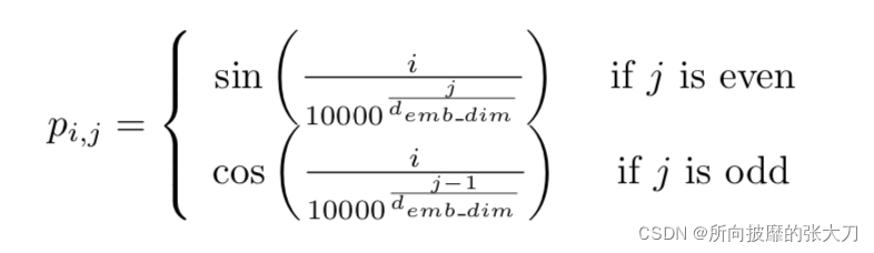
def get_positional_embeddings(sequence_length, d):
    result = torch.ones(sequence_length, d)
    for i in range(sequence_length):
        for j in range(d):
            result[i][j] = np.sin(i / (10000 ** (j / d))) if j % 2 == 0 else np.cos(i / (10000 ** ((j - 1) / d)))
    return resul

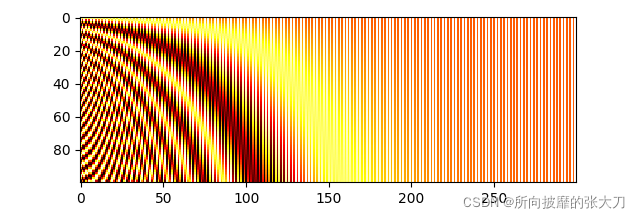
プロットされたヒートマップから、すべての「水平線」が互いに異なっていることがわかり、サンプルの位置を区別できます。

線形マッピングとカテゴリ マーカーの追加後に、位置エンコーディングをモデルに追加できるようになりました。

class MyViT(nn.Module):
    def __init__(self, input_shape, n_patches=7, hidden_d=8, n_heads=2, out_d=10):
        # Super constructor
        super(MyViT, self).__init__()

        # Input and patches sizes
        self.input_shape = input_shape
        self.n_patches = n_patches
        self.n_heads = n_heads
        assert input_shape[1] % n_patches == 0, "Input shape not entirely divisible by number of patches"
        assert input_shape[2] % n_patches == 0, "Input shape not entirely divisible by number of patches"
        self.patch_size = (input_shape[1] / n_patches, input_shape[2] / n_patches)
        self.hidden_d = hidden_d

        # 1) Linear mapper
        self.input_d = int(input_shape[0] * self.patch_size[0] * self.patch_size[1])
        self.linear_mapper = nn.Linear(self.input_d, self.hidden_d)

        # 2) Classification token
        self.class_token = nn.Parameter(torch.rand(1, self.hidden_d))

        # 3) Positional embedding
        # (In forward method)



    def forward(self, images):
        # Dividing images into patches
        n, c, w, h = images.shape
        patches = images.reshape(n, self.n_patches ** 2, self.input_d)

        # Running linear layer for tokenization
        tokens = self.linear_mapper(patches)

        # Adding classification token to the tokens
        tokens = torch.stack([torch.vstack((self.class_token, tokens[i])) for i in range(len(tokens))])

        # Adding positional embedding
        tokens += get_positional_embeddings(self.n_patches ** 2 + 1, self.hidden_d).repeat(n, 1, 1)

        return tokens

トークンのサイズは (N, 50, 8) であるため、(50, 8) 位置エンコード行列を N 回繰り返す必要があります。

LN、MSA、残りの接続

これは最も複雑な手順です。最初にトークンでレイヤーの正規化を行い、次にマルチヘッド アテンション メカニズムを適用し、最後に残差接続を追加する必要があります (LN の前に入力を接続し、マルチヘッド アテンションの後に出力を接続します)。

LN

通常、LN を (N, d) 入力に適用します。ここで、d は次元です。nn.LayerNorm が複数の次元に適用できることを発見したのは、ViT に気付くまではありませんでした:

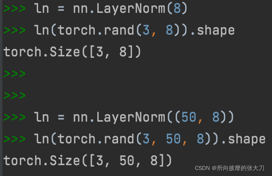
LN を介して (N, 50, 8) テンソルを実行した後、各 50x8 行列の平均値は 0 であり、標準偏差は 1 で、次元は変更されません。

多頭の自己注意

次に、アーキテクチャ図のサブグラフ c を実装する必要があります。マルチヘッド アテンション メカニズムは次のとおりです. 実装プロセスがわからない場合は [2] を参照してください. 要するに: 単一の画像の場合、他のパッチとの類似度に基づいて各パッチを更新する必要があります. 各パッチ (この例では 8 次元のベクトル) を 3 つの異なるベクトル (q、k、v (クエリ、キー、値)) に線形にマッピングします。次に、単一のパッチについて、その q ベクトルとすべての k ベクトルの間の内積を計算し、これらのベクトルの次元の平方根 d で割り、結果のソフトマックス アクティベーションを適用し、最後に計算結果を v に関連付けます。異なる k 個のベクトルのベクトル乗算、全体の計算式は次のとおりです。

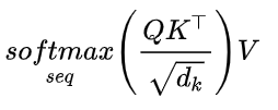
このようにして、各パッチは他のパッチとの類似性である新しい値を取得します (q、k、および v への線形マッピングの後)。プロセス全体がシングルヘッドであり、プロセス全体が複数のヘッドに対して複数回繰り返されます。すべての結果が取得された後、それらは線形レイヤーによって連結されます。

非常に多くの計算が実行されるため、MSA 用の新しいクラスを作成します。

class MyMSA(nn.Module):
    def __init__(self, d, n_heads=2):
        super(MyMSA, self).__init__()
        self.d = d
        self.n_heads = n_heads

        assert d % n_heads == 0, f"Can't divide dimension {
      
      d} into {
      
      n_heads} heads"

        d_head = int(d / n_heads)
        self.q_mappings = [nn.Linear(d_head, d_head) for _ in range(self.n_heads)]
        self.k_mappings = [nn.Linear(d_head, d_head) for _ in range(self.n_heads)]
        self.v_mappings = [nn.Linear(d_head, d_head) for _ in range(self.n_heads)]
        self.d_head = d_head
        self.softmax = nn.Softmax(dim=-1)

    def forward(self, sequences):
        # Sequences has shape (N, seq_length, token_dim)
        # We go into shape    (N, seq_length, n_heads, token_dim / n_heads)
        # And come back to    (N, seq_length, item_dim)  (through concatenation)
        result = []
        for sequence in sequences:
            seq_result = []
            for head in range(self.n_heads):
                q_mapping = self.q_mappings[head]
                k_mapping = self.k_mappings[head]
                v_mapping = self.v_mappings[head]

                seq = sequence[:, head * self.d_head: (head + 1) * self.d_head]
                q, k, v = q_mapping(seq), k_mapping(seq), v_mapping(seq)

                attention = self.softmax(q @ k.T / (self.d_head ** 0.5))
                seq_result.append(attention @ v)
            result.append(torch.hstack(seq_result))
        return torch.cat([torch.unsqueeze(r, dim=0) for r in result])

各頭部に対して、異なる Q、K、および V マッピング関数 (ここではサイズ 4x4 の正方行列) を作成することに注意してください。

入力はサイズ (N, 50, 8) のシーケンスであるため、2 つのヘッドを使用するため、ある時点で nn.Linear(4, 4 ) モジュールを使用して (N, 50, 2, 4) テンソルを持つことになります。 、連結後に (N, 50, 8) テンソルに戻ります。また、ループを使用することは、マルチヘッドの自己注意を計算する最も効率的な方法ではありませんが、コードはより簡潔になります。

残りの接続

元の (N, 50, 8) テンソルを LN と MSA の後に取得された (N, 50, 8) に追加する残留接続が追加されます。

class MyViT(nn.Module):
    def __init__(self, input_shape, n_patches=7, hidden_d=8, n_heads=2, out_d=10):
        # Super constructor
        super(MyViT, self).__init__()

        # Input and patches sizes
        self.input_shape = input_shape
        self.n_patches = n_patches
        self.n_heads = n_heads
        assert input_shape[1] % n_patches == 0, "Input shape not entirely divisible by number of patches"
        assert input_shape[2] % n_patches == 0, "Input shape not entirely divisible by number of patches"
        self.patch_size = (input_shape[1] / n_patches, input_shape[2] / n_patches)
        self.hidden_d = hidden_d

        # 1) Linear mapper
        self.input_d = int(input_shape[0] * self.patch_size[0] * self.patch_size[1])
        self.linear_mapper = nn.Linear(self.input_d, self.hidden_d)

        # 2) Classification token
        self.class_token = nn.Parameter(torch.rand(1, self.hidden_d))

        # 3) Positional embedding
        # (In forward method)

        # 4a) Layer normalization 1
        self.ln1 = nn.LayerNorm((self.n_patches ** 2 + 1, self.hidden_d))

        # 4b) Multi-head Self Attention (MSA) and classification token
        self.msa = MyMSA(self.hidden_d, n_heads)



    def forward(self, images):
        # Dividing images into patches
        n, c, w, h = images.shape
        patches = images.reshape(n, self.n_patches ** 2, self.input_d)

        # Running linear layer for tokenization
        tokens = self.linear_mapper(patches)

        # Adding classification token to the tokens
        tokens = torch.stack([torch.vstack((self.class_token, tokens[i])) for i in range(len(tokens))])

        # Adding positional embedding
        tokens += get_positional_embeddings(self.n_patches ** 2 + 1, self.hidden_d).repeat(n, 1, 1)

        # TRANSFORMER ENCODER BEGINS ###################################
        # NOTICE: MULTIPLE ENCODER BLOCKS CAN BE STACKED TOGETHER ######
        # Running Layer Normalization, MSA and residual connection
        out = tokens + self.msa(self.ln1(tokens))

        return out 

モデルを介して MNIST のランダムな (3、1、28、28) 画像を実行しても、形状 (3、50、8) の結果が得られることに注意してください。

LN、MLP、および残りの接続

次のネットワークに進み、現在のテンソルを別の LN と MLP を介して渡し、残差を介して接続します。ええと、このように構築します。

class MyViT(nn.Module):
    def __init__(self, input_shape, n_patches=7, hidden_d=8, n_heads=2, out_d=10):
        # Super constructor
        super(MyViT, self).__init__()

        # Input and patches sizes
        self.input_shape = input_shape
        self.n_patches = n_patches
        self.n_heads = n_heads
        assert input_shape[1] % n_patches == 0, "Input shape not entirely divisible by number of patches"
        assert input_shape[2] % n_patches == 0, "Input shape not entirely divisible by number of patches"
        self.patch_size = (input_shape[1] / n_patches, input_shape[2] / n_patches)
        self.hidden_d = hidden_d

        # 1) Linear mapper
        self.input_d = int(input_shape[0] * self.patch_size[0] * self.patch_size[1])
        self.linear_mapper = nn.Linear(self.input_d, self.hidden_d)

        # 2) Classification token
        self.class_token = nn.Parameter(torch.rand(1, self.hidden_d))

        # 3) Positional embedding
        # (In forward method)

        # 4a) Layer normalization 1
        self.ln1 = nn.LayerNorm((self.n_patches ** 2 + 1, self.hidden_d))

        # 4b) Multi-head Self Attention (MSA) and classification token
        self.msa = MyMSA(self.hidden_d, n_heads)

        # 5a) Layer normalization 2
        self.ln2 = nn.LayerNorm((self.n_patches ** 2 + 1, self.hidden_d))

        # 5b) Encoder MLP
        self.enc_mlp = nn.Sequential(
            nn.Linear(self.hidden_d, self.hidden_d),
            nn.ReLU()
        )


    def forward(self, images):
        # Dividing images into patches
        n, c, w, h = images.shape
        patches = images.reshape(n, self.n_patches ** 2, self.input_d)

        # Running linear layer for tokenization
        tokens = self.linear_mapper(patches)

        # Adding classification token to the tokens
        tokens = torch.stack([torch.vstack((self.class_token, tokens[i])) for i in range(len(tokens))])

        # Adding positional embedding
        tokens += get_positional_embeddings(self.n_patches ** 2 + 1, self.hidden_d).repeat(n, 1, 1)

        # TRANSFORMER ENCODER BEGINS ###################################
        # NOTICE: MULTIPLE ENCODER BLOCKS CAN BE STACKED TOGETHER ######
        # Running Layer Normalization, MSA and residual connection
        out = tokens + self.msa(self.ln1(tokens))

        # Running Layer Normalization, MLP and residual connection
        out = out + self.enc_mlp(self.ln2(out))
        # TRANSFORMER ENCODER ENDS   ###################################

        return out 

このように、モデルがランダムな (3, 1, 28, 28) 画像テンソルを入力した場合、out 出力は引き続き (3, 50, 8) テンソルを取得します。

分類MLP

最後に、カテゴリ ラベルが追加された場所に対応する N シーケンスからカテゴリ マーカー (最初のマーカー) のみを抽出し、各マーカーを使用して N カテゴリを取得できます。

各トークンは 8 次元のベクトルであると判断し、可能な数は 10 であるため、分類 MLP を単純な 8x10 行列として実装し、SoftMax 関数のアクティベーションを使用できます。

class MyViT(nn.Module):
    def __init__(self, input_shape, n_patches=7, hidden_d=8, n_heads=2, out_d=10):
        # Super constructor
        super(MyViT, self).__init__()

        # Input and patches sizes
        self.input_shape = input_shape
        self.n_patches = n_patches
        self.n_heads = n_heads
        assert input_shape[1] % n_patches == 0, "Input shape not entirely divisible by number of patches"
        assert input_shape[2] % n_patches == 0, "Input shape not entirely divisible by number of patches"
        self.patch_size = (input_shape[1] / n_patches, input_shape[2] / n_patches)
        self.hidden_d = hidden_d

        # 1) Linear mapper
        self.input_d = int(input_shape[0] * self.patch_size[0] * self.patch_size[1])
        self.linear_mapper = nn.Linear(self.input_d, self.hidden_d)

        # 2) Classification token
        self.class_token = nn.Parameter(torch.rand(1, self.hidden_d))

        # 3) Positional embedding
        # (In forward method)

        # 4a) Layer normalization 1
        self.ln1 = nn.LayerNorm((self.n_patches ** 2 + 1, self.hidden_d))

        # 4b) Multi-head Self Attention (MSA) and classification token
        self.msa = MyMSA(self.hidden_d, n_heads)

        # 5a) Layer normalization 2
        self.ln2 = nn.LayerNorm((self.n_patches ** 2 + 1, self.hidden_d))

        # 5b) Encoder MLP
        self.enc_mlp = nn.Sequential(
            nn.Linear(self.hidden_d, self.hidden_d),
            nn.ReLU()
        )

        # 6) Classification MLP
        self.mlp = nn.Sequential(
            nn.Linear(self.hidden_d, out_d),
            nn.Softmax(dim=-1)
        )

    def forward(self, images):
        # Dividing images into patches
        n, c, w, h = images.shape
        patches = images.reshape(n, self.n_patches ** 2, self.input_d)

        # Running linear layer for tokenization
        tokens = self.linear_mapper(patches)

        # Adding classification token to the tokens
        tokens = torch.stack([torch.vstack((self.class_token, tokens[i])) for i in range(len(tokens))])

        # Adding positional embedding
        tokens += get_positional_embeddings(self.n_patches ** 2 + 1, self.hidden_d).repeat(n, 1, 1)

        # TRANSFORMER ENCODER BEGINS ###################################
        # NOTICE: MULTIPLE ENCODER BLOCKS CAN BE STACKED TOGETHER ######
        # Running Layer Normalization, MSA and residual connection
        out = tokens + self.msa(self.ln1(tokens))

        # Running Layer Normalization, MLP and residual connection
        out = out + self.enc_mlp(self.ln2(out))
        # TRANSFORMER ENCODER ENDS   ###################################

        # Getting the classification token only
        out = out[:, 0]

        return self.mlp(out)

モデルの出力は (N, 10) テンソルになりました。よし、完了です！

次に、モデルがどのように機能するかを見てみましょう。Torch シードを手動で設定し (0 に設定)、CPU で実行します。

エピローグ

オリジナルの ViT の作成者は、GeLU アクティベーション関数、多層 MLP、およびスタックされた複数の Transformer エンコーダ ブロックを一緒に使用しました。これは最も単純な物乞いバージョンです. 後でこれに基づいて追加できます. 公式アカウントをフォローして「vit」と返信すると、完全なコードを取得できます.

---

論文: https://arxiv.org/abs/2010.11929
参照:
[1] https://zhuanlan.zhihu.com/p/342261872
[2] https://zhuanlan.zhihu.com/p/340149804

より多くのコンテンツに注意を払うことを歓迎します: