https://github.com/waleedka/traffic-signs-tensorflow
交通標識分類-tensorflow実装から分類および翻訳
テストプラットフォームはwin10システム、python3オペレーティング環境であり、tensorflow-gpuを構成する必要があります。
まず、必要なライブラリを紹介します
import os
import random
import skimage.data
import skimage.transform
import matplotlib
import matplotlib.pyplot as plt
import numpy as np
import tensorflow as tf

# Allow image embeding in notebook
%matplotlib inline
データセット分析
データディレクトリ構造:
/traffic/datasets/BelgiumTS/Training/
/traffic/datasets/BelgiumTS/Testing/
トレーニングセットとテストセットの下には62のサブディレクトリがあり、名前の範囲は00000から00061です。
カタログの名前は0から61までのタグを表し、各カタログの画像はそのタグに属する交通標識を表します。
画像の保存形式は.ppm形式で、skimageライブラリを使用して読み取ることができます。
def load_data(data_dir):
    """Loads a data set and returns two lists:

    images: a list of Numpy arrays, each representing an image.
    labels: a list of numbers that represent the images labels.
    """
    # Get all subdirectories of data_dir. Each represents a label.
    directories = [d for d in os.listdir(data_dir)
                   if os.path.isdir(os.path.join(data_dir, d))]
    # Loop through the label directories and collect the data in
    # two lists, labels and images.
    labels = []
    images = []
    for d in directories:
        label_dir = os.path.join(data_dir, d)
        file_names = [os.path.join(label_dir, f)
                      for f in os.listdir(label_dir) if f.endswith(".ppm")]
        # For each label, load it's images and add them to the images list.
        # And add the label number (i.e. directory name) to the labels list.
        for f in file_names:
            images.append(skimage.data.imread(f))
            labels.append(int(d))
    return images, labels

# Load training and testing datasets.
ROOT_PATH = ""
train_data_dir = os.path.join(ROOT_PATH, "datasets/BelgiumTS/Training")
test_data_dir = os.path.join(ROOT_PATH, "datasets/BelgiumTS/Testing")

images, labels = load_data(train_data_dir)
すべての写真とラベルの数を印刷します
print("Unique Labels: {0}\nTotal Images: {1}".format(len(set(labels)),
len(images)))
Unique Labels: 62
Total Images: 4575
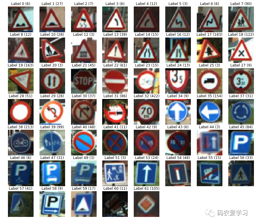
各タイプのラベルの最初の画像を表示します
def display_images_and_labels(images, labels):
    """Display the first image of each label."""
    unique_labels = set(labels) # set:不重复出现
    plt.figure(figsize=(15, 15)) # figure size
    i = 1
    for label in unique_labels:
        # Pick the first image for each label.
        image = images[labels.index(label)] #每个label在整个labels表中的位置
        # str1.index(str2, beg=0, end=len(string)) str2在str1中的索引值
        # print(labels.index(label))
        plt.subplot(8, 8, i)  # A grid of 8 rows x 8 columns
        plt.axis('off')
        plt.title("Label {0} ({1})".format(label, labels.count(label)))# label,totalnum
        i += 1
        _ = plt.imshow(image)
    plt.show()

display_images_and_labels(images, labels)
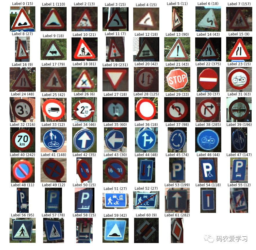
画像は正方形ですが、各画像のアスペクト比は異なります。ニューラルネットワークの入力サイズは固定されているため、いくつかの処理を行う必要があります。処理する前にラベルの写真を撮り、次のように、ラベル32などのラベルの下にある写真をさらにいくつか見てください。
def display_label_images(images, label):
    """Display images of a specific label."""
    limit = 24  # show a max of 24 images
    plt.figure(figsize=(15, 5))
    i = 1

    start = labels.index(label)
    end = start + labels.count(label)# count:统计字符串里某个字符出现的次数
    for image in images[start:end][:limit]:
        plt.subplot(3, 8, i)  # 3 rows, 8 per row
        plt.axis('off')
        i += 1
        plt.imshow(image)
    plt.show()

display_label_images(images, 32)
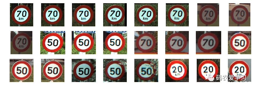
上の写真から、制限速度は異なりますが、すべて同じカテゴリにグループ化されていることがわかります。これは非常に良いことです。後続の手順では数値の概念を無視できます。これが、データセットを事前に理解することが非常に重要であり、その後の作業で多くの苦痛と混乱を避けることができる理由です。
では、元の画像のサイズはどれくらいですか?最初にいくつか印刷してみましょう:(
ヒント:min()とmax()の値を印刷します。これは、データの範囲を確認し、エラーを早期に見つける簡単な方法です)
for image in images[:5]:
    print("shape: {0}, min: {1}, max: {2}".format(image.shape, image.min(),
            image.max()))
shape: (141, 142, 3), min: 0, max: 255
shape: (120, 123, 3), min: 0, max: 255
shape: (105, 107, 3), min: 0, max: 255
shape: (94, 105, 3), min: 7, max: 255
shape: (128, 139, 3), min: 0, max: 255
画像のサイズは約128128です。このサイズを使用して画像を保存できるため、できるだけ多くの情報を保存できます。ただし、初期の開発では、より小さなサイズを使用すると、トレーニングモデルが高速になり、より高速に反復できます。
サイズは3232を選択してください。肉眼で画像を認識しやすく(下の画像を参照)、縮小率が128 * 128の倍数になるようにします。
# Resize images
images32 = [skimage.transform.resize(image, (32, 32))
                for image in images]
display_images_and_labels(images32, labels)
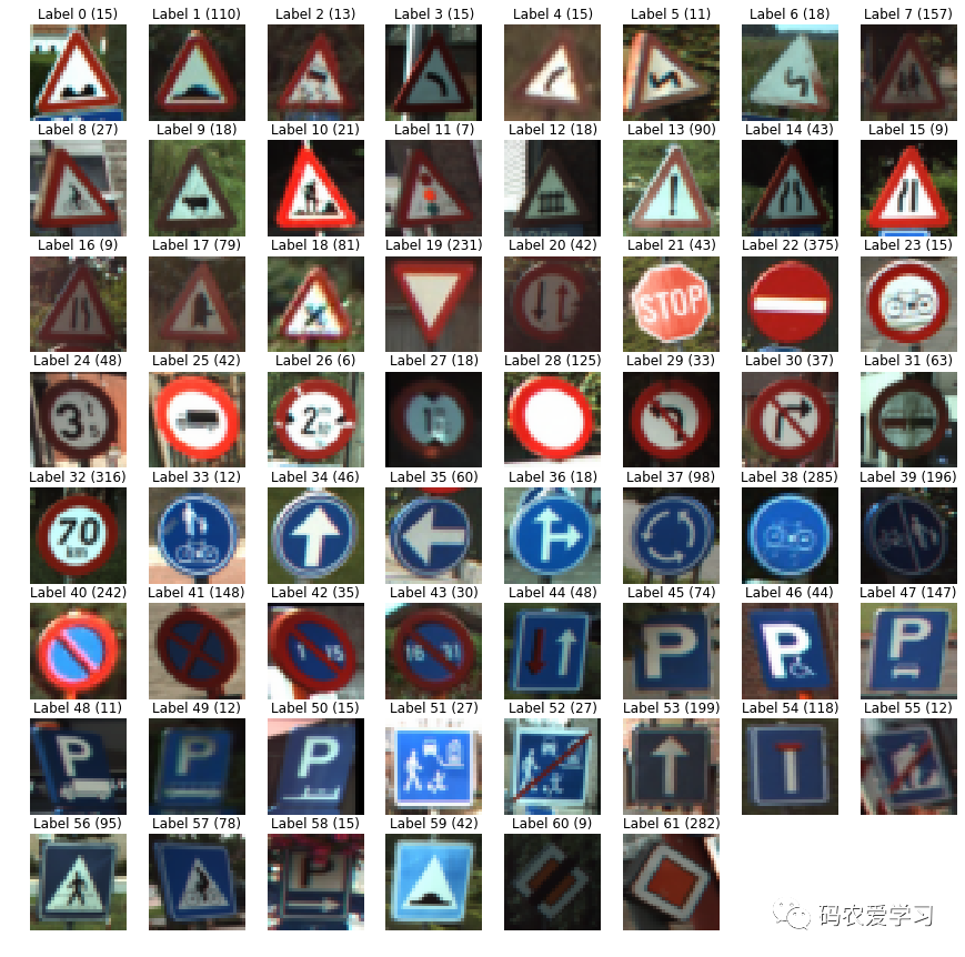
32x32の画像はそれほど鮮明ではありませんが、それでも認識できます。matplotlibライブラリが画像をグリッドサイズに一致させようとするため、上の表示には実際のサイズよりも大きい画像が表示されることに注意してください。
いくつかの画像のサイズを印刷して、正しいことを確認しましょう。
for image in images32[:5]:
    print("shape: {0}, min: {1}, max: {2}".format(image.shape, image.min(), image.max()))
shape: (32, 32, 3), min: 0.03529411764705882, max: 0.996078431372549
shape: (32, 32, 3), min: 0.033953737745098134, max: 0.996078431372549
shape: (32, 32, 3), min: 0.03694182751225489, max: 0.996078431372549
shape: (32, 32, 3), min: 0.06460056678921595, max: 0.9191425398284313
shape: (32, 32, 3), min: 0.06035539215686279, max: 0.9028492647058823
サイズは正しいです。ただし、最小値と最大値を確認してください。これらの範囲は0〜1.0になりました。これは、上記の0〜255の範囲とは異なります。スケーリング関数がこの変換を行います。値を0〜1.0の範囲に正規化することは非常に一般的であるため、これを維持します。ただし、画像を通常の0〜255の範囲に戻す場合は、255を掛けることを忘れないでください。
labels_a = np.array(labels) # 标签
images_a = np.array(images32) # 图片
print("labels: ", labels_a.shape, "\nimages: ", images_a.shape)
labels:  (4575,)
images:  (4575, 32, 32, 3)
モデル構築
まず、Graphオブジェクトを作成します。
次に、画像とラベルを配置するためのプレースホルダー(プレースホルダー)を設定します。プレースホルダーは、TensorFlowがメインプログラムから入力を受け取る方法です。
パラメータimages_phの次元は[None、32、32、3]です。これらの4つのパラメータは、[バッチサイズ、高さ、幅、チャネル](通常はNHWCと略されます)を表します。バッチサイズはNoneで表されます。これは、バッチサイズが柔軟であることを意味します。つまり、コードを変更せずに、任意のバッチサイズのデータをモデルにインポートできます。
完全に接続された層の出力は、長さ62の対数ベクトルです。出力データは次のようになります:[0.3、0、0、1.2、2.1、0.01、0.4、... ...、0、0]。値が高いほど、画像がラベルを表す可能性が高くなります。出力は確率ではなく、任意の値にすることができ、加算の結果は1に等しくありません。出力ニューロンの実際の値は重要ではありません。これは、62個のニューロンに対する相対値にすぎないためです。必要に応じて、softmax関数または他の関数を簡単に使用して確率に変換できます(ここでは必要ありません)。
このプロジェクトでは、最大値に対応するインデックスが画像の分類ラベルを表すため、このインデックスを知る必要があるだけです。argmax関数の出力結果は、[0、61]の範囲の整数になります。
クロスエントロピーは分類問題に適しており、差の2乗は回帰問題に適しているため、損失関数はクロスエントロピー計算方法を使用します。
クロスエントロピーは、2つの確率ベクトル間の差の尺度です。したがって、ニューラルネットワークのラベルと出力を確率ベクトルに変換する必要があります。この操作を実現するために、TensorFlowにはsparse_softmax_cross_entropy_with_logits関数があります。この関数は、ニューラルネットワークのラベルと出力を入力パラメーターとして受け取り、3つのことを行います。1つはラベルの次元を[なし、62](これは0-1ベクトル)に変換します。2つ目はsoftmaxを使用します。ラベルデータとニューラルネットワークの出力結果は確率値に変換されます。3番目に、2つの間のクロスエントロピーが計算されます。この関数は、次元[None]のベクトルを返します(ベクトルの長さはバッチサイズです)。次に、reduce_mean関数を使用して、最終的な損失値を表す値を取得します。
モデルパラメータの調整には、勾配降下アルゴリズムが使用されます。実験後の学習率は0.08がより適切であり、反復は800回です。
# Create a graph to hold the model.
graph = tf.Graph()

# Create model in the graph.
with graph.as_default():
    # Placeholders for inputs and labels.
    images_ph = tf.placeholder(tf.float32, [None, 32, 32, 3])
    labels_ph = tf.placeholder(tf.int32, [None])

    # Flatten input from: [None, height, width, channels]
    # To: [None, height * width * channels] == [None, 3072]
    images_flat = tf.contrib.layers.flatten(images_ph)

    # Fully connected layer. 【全连接层】
    # Generates logits of size [None, 62]
    logits = tf.contrib.layers.fully_connected(images_flat, 62, tf.nn.relu)

    # Convert logits to label indexes (int).
    # Shape [None], which is a 1D vector of length == batch_size.
    predicted_labels = tf.argmax(logits, 1)

    # Define the loss function. 【损失函数】
    # Cross-entropy is a good choice for classification. 交叉熵
    loss = tf.reduce_mean(tf.nn.sparse_softmax_cross_entropy_with_logits(logits=logits, labels=labels_ph))

    # Create training op.  【梯度下降算法】
    train = tf.train.GradientDescentOptimizer(learning_rate=0.08).minimize(loss)

    # And, finally, an initialization op to execute before training.
    # TODO: rename to tf.global_variables_initializer() on TF 0.12.
    init = tf.global_variables_initializer()

print("images_flat: ", images_flat)
print("logits: ", logits)
print("loss: ", loss)
print("predicted_labels: ", predicted_labels)
print(tf.nn.sparse_softmax_cross_entropy_with_logits(logits=logits, labels=labels_ph))
images_flat:  Tensor("Flatten/flatten/Reshape:0", shape=(?, 3072), dtype=float32)
logits:  Tensor("fully_connected/Relu:0", shape=(?, 62), dtype=float32)
loss:  Tensor("Mean:0", shape=(), dtype=float32)
predicted_labels:  Tensor("ArgMax:0", shape=(?,), dtype=int64)
Tensor("SparseSoftmaxCrossEntropyWithLogits_1/SparseSoftmaxCrossEntropyWithLogits:0", shape=(?,), dtype=float32)
トレーニング
# Create a session to run the graph we created.
session = tf.Session(graph=graph)

# First step is always to initialize all variables.
# We don't care about the return value, though. It's None.
_ = session.run([init])
for i in range(801):
    _, loss_value = session.run([train, loss],
                                feed_dict={images_ph: images_a, labels_ph: labels_a})
    if i % 20 == 0:
        print("Loss: ", loss_value)
Loss:  4.237691
Loss:  3.4573376
Loss:  3.081502
Loss:  2.89802
Loss:  2.780877
Loss:  2.6962612
Loss:  2.6338725
Loss:  2.5843806
Loss:  2.5426073
Loss:  2.5067272
Loss:  2.47533
Loss:  2.4474416
Loss:  2.4224002
Loss:  2.399726
Loss:  2.3790603
Loss:  2.360102
Loss:  2.3426225
Loss:  2.3264341
Loss:  2.3113735
Loss:  2.2973058
Loss:  2.2841291
Loss:  2.2717524
Loss:  2.2600884
Loss:  2.248851
Loss:  2.2366288
Loss:  2.2220945
Loss:  2.2083163
Loss:  2.1957521
Loss:  2.184217
Loss:  2.1736012
Loss:  2.1637862
Loss:  2.1546829
Loss:  2.1461952
Loss:  2.1382334
Loss:  2.13073
Loss:  2.1236277
Loss:  2.1168776
Loss:  2.1104405
Loss:  2.104286
Loss:  2.0983875
Loss:  2.0927253
トレーニング済みモデルを使用する-トレーニングセットの精度をテストする
セッションオブジェクト(セッション)には、モデル内のすべての変数の値(つまり重み)が含まれています。
# 随机从训练集中选取10张图片
sample_indexes = random.sample(range(len(images32)), 10)
sample_images = [images32[i] for i in sample_indexes]
sample_labels = [labels[i] for i in sample_indexes]

# Run the "predicted_labels" op.
predicted = session.run([predicted_labels],
                        feed_dict={images_ph: sample_images})[0]
print(sample_labels)#样本标签
print(predicted)#预测值
[20, 49, 18, 38, 22, 61, 19, 58, 17, 19]
[28 47 18 38 18 60 19 47 17 19]
# Display the predictions and the ground truth visually.
fig = plt.figure(figsize=(10, 10))
for i in range(len(sample_images)):
    truth = sample_labels[i]
    prediction = predicted[i]
    plt.subplot(5, 2,1+i)
    plt.axis('off')
    color='green' if truth == prediction else 'red'
    plt.text(40, 10, "Truth:        {0}\nPrediction: {1}".format(truth, prediction),
             fontsize=12, color=color)
    plt.imshow(sample_images[i])
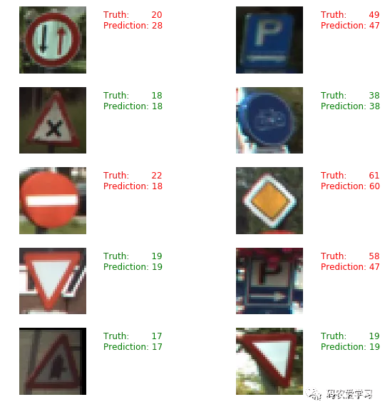
上の図の真実の後の数字は実際のラベルであり、予測の後の数字は予測されたラベルです。
現在の分類テストはまだトレーニングセットの写真であるため、未知のデータセットでモデルがどのように実行されるかはわかりません。
次に、テストセットで評価します。
モデル評価-テストセットの精度を検証します
視覚化の結果は非常に直感的ですが、モデルの精度を測定するには、より正確な方法が必要です。ここで、検証セットが役立ちます。
# 加载测试集图片
test_images, test_labels = load_data(test_data_dir)
# 转换图片尺寸
test_images32 = [skimage.transform.resize(image, (32, 32))
                 for image in test_images]
#显示转换后的图片
display_images_and_labels(test_images32, test_labels)
# Run predictions against the full test set.
predicted = session.run([predicted_labels],
                        feed_dict={images_ph: test_images32})[0]
# 计算准确度
match_count = sum([int(y == y_) for y, y_ in zip(test_labels, predicted)])
accuracy = match_count / len(test_labels)
# 输出测试集上的准确度
print("Accuracy: {:.3f}".format(accuracy))
Accuracy: 0.534
# Close the session. This will destroy the trained model.
session.close()