TensorFlow-VGG16モデルの再現

1VGGの概要

VGGのフルネームは、オックスフォード大学のオックスフォードビジュアルジオメトリグループを指します。2014年のImageNetチャレンジでは、このグループによって設計されたVGGニューラルネットワークモデルが、ポジショニングおよび分類追跡コンテストで1位と2位を獲得しました。

• VGG紙

大規模な画像認識のための非常に深い畳み込みネットワーク

その主な貢献は、3 * 3の小さな畳み込みカーネルのネットワーク構造を使用して徐々に深くなるネットワークの包括的な評価にあると指摘しています。結果は、ネットワークの深さを16〜19層に深くすることで、以前のネットワークを大幅に超えることができることを示しています。構造。

1.1VGGの構造特性

• トレーニング入力：固定サイズ224 * 224RGB画像

• 前処理：各ピクセル値からトレーニングセットのRGB平均値を減算します

• 畳み込みカーネル：ステップサイズ1でスタックされた一連の3 * 3畳み込みカーネル。パディングを使用して、畳み込み後の画像の空間解像度を変更しません。

• 空間プーリング：畳み込み「ヒープ」に続く最大プーリング。これは、2 * 2のスライディングウィンドウであり、ステップサイズは2です。

• 完全に接続された層：特徴抽出が完了した後、3つの完全に接続された層が接続され、最初の2つは4096チャネル、3つ目は1000チャネル、最後は確率を出力するソフトマックス層です。

• すべての隠れ層は非線形補正ReLuを使用します

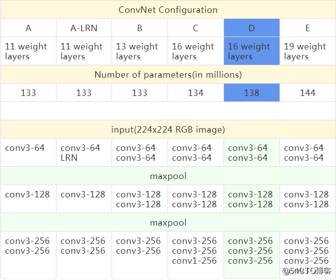
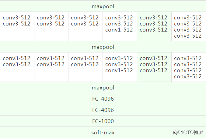
1.2詳細な構成

表の各列は異なるネットワークを表しており、深さのみが異なります（レイヤー数の計算にはプーリングレイヤーは含まれません）。畳み込みのチャネル数は非常に少なく、最初の層には64チャネルしかありません。最大プーリング後、チャネル数は512チャネルに達するまで2倍になります。
各モデルのパラメータ数を比較すると、ネットワークは深くなっていますが、パラメータ数は主に完全に接続された層に集中しているため、重みは大幅に増加していません。
最後の2列（列Dと列E）は、VGG-16とVGG-19のより優れたモデル構造です。この記事では、TensorFlowコードを使用してVGG-16モデルを再現し、トレーニング済みのモデルパラメーターファイルを使用して画像オブジェクトを分類します。テスト。

1.3論文で紹介されたトレーニング方法

• トレーニング方法は、マルチスケールトレーニング画像のサンプリング方法に一貫性がないことを除いて、基本的にAlexNetと同じです。

• トレーニングはミニバッチ勾配降下法を採用し、バッチサイズ= 256

• 運動量最適化アルゴリズムを使用して、運動量= 0.9

• L2正則化法を採用し、ペナルティ係数は0.00005、ドロップアウト率は0.5に設定しています。

• 初期学習率は0.001です。検証セットの精度が向上しなくなると、学習率は元の0.1倍に低下し、合計3回低下します。

• 反復の総数は370K（74エポック）です

• データエンハンスメントは、ランダムトリミング、水平フリップ、RGBカラー変更を採用しています

• トレーニング画像のサイズを設定する2つの方法（等方性スケーリング後のトレーニング画像の最小エッジを表すようにSを定義します）。

• 最初の方法は、シングルサイズの画像トレーニング（S = 256または384）であり、入力画像は224 * 224サイズの画像からランダムにトリミングされます。原則として、Sは224以上の任意の値を取ることができます。

• 2番目の方法はマルチスケールトレーニングです。各画像は[Smin、Smax]からランダムに選択されてサイズがスケーリングされます。画像内のターゲットオブジェクトのサイズは可変であるため、この方法はトレーニングに効果的であり、Aサイズと見なすことができます。 -ジッタートレーニングセットデータの強化

ネットワークの重みの初期化は非常に重要であると論文で述べられています。深いネットワークの勾配が不安定であるため、不適切な初期化はネットワークの学習を妨げます。したがって、最初に浅いネットワークをトレーニングしてから、トレーニングした浅いネットワークを使用して深いネットワークを初期化します。

2VGG-16ネットワークの複製

2.1 VGG-16ネットワーク構造（順伝播）再現

VGG-16の16層ネットワーク構造を再現し、Vgg16クラスにカプセル化します。ここではトレーニング済みのvgg16.npyパラメータファイルを使用していることに注意してください。モデルを自分でトレーニングする必要はないため、トレーニングする必要はありません。トレーニングファイルを作成します。逆伝播関数。テスト用に順方向伝播部分を作成するだけです。

以下のコードに詳細なコメントを追加し、各レイヤーのネットワークの構造とサイズの情報を出力するためのprintステートメントをいくつか追加しました。

vgg16.py

import inspect
import os
import numpy as np
import tensorflow as tf
import time
import matplotlib.pyplot as plt

VGG_MEAN = [103.939, 116.779, 123.68] # 样本RGB的平均值

class Vgg16():
    def __init__(self, vgg16_path=None):
        if vgg16_path is None:
            # os.getcwd()方法用于返回当前工作目录(npy模型参数文件)
            vgg16_path = os.path.join(os.getcwd(), "vgg16.npy")
            print("path(vgg16.npy):",vgg16_path)
            # 遍历其内键值对，导入模型参数
            self.data_dict = np.load(vgg16_path, encoding='latin1').item()
        for x in self.data_dict: # 遍历datat_dict中的每个键
            print("key in data_dict:",x)

    def forward(self, images):

        print("build model started...")
        start_time = time.time() # 获取前向传播的开始时间
        rgb_scaled = images * 255.0 # 逐像素乘以255
        # 从GRB转换色彩通道到BGR
        red, green, blue = tf.split(rgb_scaled,3,3)
        # assert是加入断言，用断每个操作后的维度变化是否和预期一致
        assert red.get_shape().as_list()[1:] == [224, 224, 1]
        assert green.get_shape().as_list()[1:] == [224, 224, 1]
        assert blue.get_shape ().as_list()[1:] == [224, 224, 1]

        bgr = tf.concat([     
            blue - VGG_MEAN[0],
            green - VGG_MEAN[1],
            red - VGG_MEAN[2]],3)
        assert bgr.get_shape().as_list()[1:] == [224, 224, 3]

        #构建VGG的16层网络（包含5段(2+2+3+3+3=13)卷积，3层全连接）
        # 第1段，2卷积层+最大池化层
        print("==>input image shape:",bgr.get_shape().as_list())
        self.conv1_1 = self.conv_layer(bgr, "conv1_1")
        print("=>after conv1_1 shape:",self.conv1_1.get_shape().as_list())
        self.conv1_2 = self.conv_layer(self.conv1_1, "conv1_2")
        print("=>after conv1_2 shape:",self.conv1_2.get_shape().as_list())
        self.pool1 = self.max_pool_2x2(self.conv1_2, "pool1")
        print("---after pool1 shape:",self.pool1.get_shape().as_list())

        # 第2段，2卷积层+最大池化层
        self.conv2_1 = self.conv_layer(self.pool1, "conv2_1")
        print("=>after conv2_1 shape:",self.conv2_1.get_shape().as_list())
        self.conv2_2 = self.conv_layer(self.conv2_1, "conv2_2")
        print("=>after conv2_2 shape:",self.conv2_2.get_shape().as_list())
        self.pool2 = self.max_pool_2x2(self.conv2_2, "pool2")
        print("---after pool2 shape:",self.pool2.get_shape().as_list())

        # 第3段，3卷积层+最大池化层
        self.conv3_1 = self.conv_layer(self.pool2, "conv3_1")
        print("=>after conv3_1 shape:",self.conv3_1.get_shape().as_list())
        self.conv3_2 = self.conv_layer(self.conv3_1, "conv3_2")
        print("=>after conv3_2 shape:",self.conv3_2.get_shape().as_list())
        self.conv3_3 = self.conv_layer(self.conv3_2, "conv3_3")
        print("=>after conv3_3 shape:",self.conv3_3.get_shape().as_list())
        self.pool3 = self.max_pool_2x2(self.conv3_3, "pool3")
        print("---after pool3 shape:",self.pool3.get_shape().as_list())

        # 第4段，3卷积层+最大池化层
        self.conv4_1 = self.conv_layer(self.pool3, "conv4_1")
        print("=>after conv4_1 shape:",self.conv4_1.get_shape().as_list())
        self.conv4_2 = self.conv_layer(self.conv4_1, "conv4_2")
        print("=>after conv4_2 shape:",self.conv4_2.get_shape().as_list())
        self.conv4_3 = self.conv_layer(self.conv4_2, "conv4_3")
        print("=>after conv4_3 shape:",self.conv4_3.get_shape().as_list())
        self.pool4 = self.max_pool_2x2(self.conv4_3, "pool4")
        print("---after pool4 shape:",self.pool4.get_shape().as_list())

        # 第5段，3卷积层+最大池化层
        self.conv5_1 = self.conv_layer(self.pool4, "conv5_1")
        print("=>after conv5_1 shape:",self.conv5_1.get_shape().as_list())
        self.conv5_2 = self.conv_layer(self.conv5_1, "conv5_2")
        print("=>after conv5_2 shape:",self.conv5_2.get_shape().as_list())
        self.conv5_3 = self.conv_layer(self.conv5_2, "conv5_3")
        print("=>after conv5_3 shape:",self.conv5_3.get_shape().as_list())
        self.pool5 = self.max_pool_2x2(self.conv5_3, "pool5")
        print("---after pool5 shape:",self.pool5.get_shape().as_list())

        # 3层全连接层
        self.fc6 = self.fc_layer(self.pool5, "fc6") # 输出4096长度
        print("=>after fc6 shape:",self.fc6.get_shape().as_list())
        assert self.fc6.get_shape().as_list()[1:] == [4096]
        self.relu6 = tf.nn.relu(self.fc6)         
        self.fc7 = self.fc_layer(self.relu6, "fc7")
        print("=>after fc7 shape:",self.fc7.get_shape().as_list())
        self.relu7 = tf.nn.relu(self.fc7)        
        self.fc8 = self.fc_layer(self.relu7, "fc8")
        print("=>after fc8 shape:",self.fc8.get_shape().as_list())

        # softmax分类，得到属于各类别的概率
        self.prob = tf.nn.softmax(self.fc8, name="prob")

        end_time = time.time() # 得到前向传播的结束时间
        print(("forward time consuming: %f" % (end_time-start_time)))

        # 清空本次读取到的模型参数字典
        self.data_dict = None 

    # 定义卷积运算
    def conv_layer(self, x, name):
        # 根据命名空间name从参数字典(npy文件)中取到对应卷积层的网络参数
        with tf.variable_scope(name): 
            w = self.get_conv_filter(name) # 读到该层的卷积核大小
            # 卷积计算
            conv = tf.nn.conv2d(x, w, [1, 1, 1, 1], padding='SAME') 
            conv_biases = self.get_bias(name) # 读到偏置项b
            # 加上偏置，并做激活计算
            result = tf.nn.relu(tf.nn.bias_add(conv, conv_biases)) 
            return result

    # 定义获取卷积核大小的函数
    def get_conv_filter(self, name):
        # 根据命名空间name从参数字典中取到对应的卷积核大小
        return tf.constant(self.data_dict[name][0], name="filter") 

    # 定义获取偏置的函数
    def get_bias(self, name):
        # 根据命名空间name从参数字典中取到对应的偏置
        return tf.constant(self.data_dict[name][1], name="biases")

    # 定义2x2最大池化操作
    def max_pool_2x2(self, x, name):
        return tf.nn.max_pool(x, ksize=[1, 2, 2, 1], strides=[1, 2, 2, 1], padding='SAME', name=name)

    # 定义全连接层的前向传播计算
    def fc_layer(self, x, name):
        # 根据命名空间name做全连接层的计算
        with tf.variable_scope(name): 
            shape = x.get_shape().as_list() # 获取该层的维度信息列表
            print("fc_layer shape:",shape)
            dim = 1
            for i in shape[1:]:
                dim *= i # 将每层的维度相乘
            #  改变特征图的形状，将得到的多维特征做拉伸操作，只在进入第六层全连接层做该操作
            x = tf.reshape(x, [-1, dim])
            w = self.get_fc_weight(name) # 读到权重值
            b = self.get_bias(name) # 读到偏置项

            # 对该层输入做加权求和，再加上偏置
            result = tf.nn.bias_add(tf.matmul(x, w), b) 
            return result

    # 定义获取权重的函数
    def get_fc_weight(self, name):
        # 根据命名空间name从参数字典中取到对应的权重
        return tf.constant(self.data_dict[name][0], name="weights")

2.2画像読み込み表示と前処理

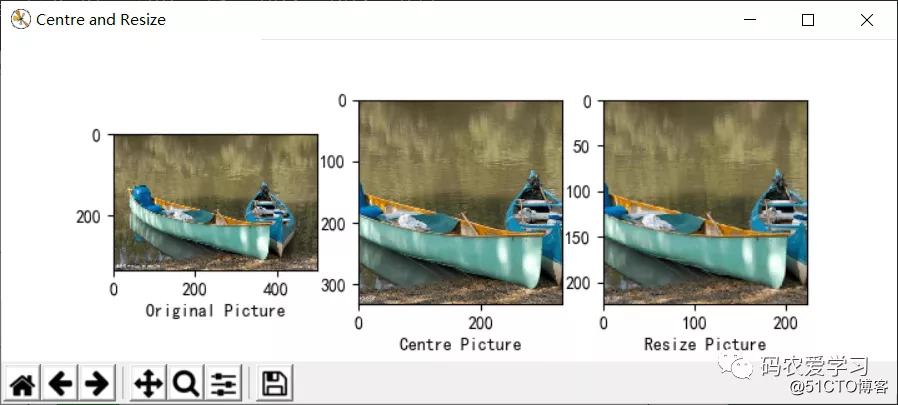
テスト画像は、必要な前処理操作（サイズのトリミング、ピクセルの正規化など）を実行し、matplotlibを使用して元の画像とテスト用に前処理された画像を表示する必要があります。

utils.py

from skimage import io, transform
import numpy as np
import matplotlib.pyplot as plt
import tensorflow as tf
from pylab import mpl

mpl.rcParams['font.sans-serif']=['SimHei'] # 正常显示中文标签
mpl.rcParams['axes.unicode_minus']=False # 正常显示正负号

# 定义加载图像、显示与预处理函数
def load_image(path):
    fig = plt.figure("Centre and Resize")
    img = io.imread(path)  # 根据传入的路径读入图片
    img = img / 255.0 # 将像素归一化到[0,1]

    # 将该画布分为一行三列
    ax0 = fig.add_subplot(131) # 把下面的图像放在该画布的第一个位置
    ax0.set_xlabel(u'Original Picture')  # 添加子标签
    ax0.imshow(img)  # 添加展示该图像

    short_edge = min(img.shape[:2]) # 找到该图像的最短边
    y = (img.shape[0] - short_edge) // 2 
    x = (img.shape[1] - short_edge) // 2  # 把图像的w和h分别减去最短边，求平均
    crop_img = img[y:y+short_edge, x:x+short_edge] # 取出切分出的中心图像

    ax1 = fig.add_subplot(132) 
    ax1.set_xlabel(u"Centre Picture") 
    ax1.imshow(crop_img) # 显示中心图像

    # resize成固定的imag_szie224x224
    re_img = transform.resize(crop_img, (224, 224)) 

    ax2 = fig.add_subplot(133) 
    ax2.set_xlabel(u"Resize Picture") 
    ax2.imshow(re_img) # 显示224x224图像

    img_ready = re_img.reshape((1, 224, 224, 3))

    return img_ready

# 定义百分比转换函数
def percent(value):
    return '%.2f%%' % (value * 100)

2.3オブジェクトタイプのリスト

このファイルは、予測結果番号に対応する実際のオブジェクトの名前を1000に保存し、最後の予測IDをオブジェクト名にマップするために使用されます。

Nclasses.py

# 每个图像的真实标签，以及对应的索引值
labels = {
 0: 'tench\n Tinca tinca',
 1: 'goldfish\n Carassius auratus',
 2: 'great white shark\n white shark\n man-eater\n man-eating shark\n Carcharodon carcharias',
 3: 'tiger shark\n Galeocerdo cuvieri',
 4: 'hammerhead\n hammerhead shark',
 5: 'electric ray\n crampfish\n numbfish\n torpedo',
 6: 'stingray',
 7: 'cock',
 8: 'hen',
 9: 'ostrich\n Struthio camelus',
 ...省略
 993: 'gyromitra',
 994: 'stinkhorn\n carrion fungus',
 995: 'earthstar',
 996: 'hen-of-the-woods\n hen of the woods\n Polyporus frondosus\n Grifola frondosa',
 997: 'bolete',
 998: 'ear\n spike\n capitulum',
 999: 'toilet tissue\n toilet paper\n bathroom tissue'}

2.4オブジェクト分類テストインターフェース機能

テスト画像のロード、モデル操作の呼び出し、予測結果の表示などに使用されるインターフェイス関数を記述します。

app.py

import numpy as np
import tensorflow as tf
import matplotlib.pyplot as plt
import vgg16
import utils
from Nclasses import labels

img_path = input('Input the path and image name:')
img_ready = utils.load_image(img_path) # 调用自定义的load_image()函数

# 定义一个figure画图窗口，并指定窗口的名称
fig=plt.figure(u"Top-5 预测结果") 

with tf.Session() as sess:
    # 定义一个维度为[1,224,224,3], 类型为float32的tensor占位符
    images = tf.placeholder(tf.float32, [1, 224, 224, 3])
    vgg = vgg16.Vgg16() # 自定义的Vgg16类实例化出vgg对象
    # 调用类的成员方法forward()，并传入待测试图像，也就是网络前向传播的过程
    vgg.forward(images)
    # 将一个batch的数据喂入网络，得到网络的预测输出
    probability = sess.run(vgg.prob, feed_dict={images:img_ready})
    # np.argsort返回预测值由小到大的索引值，并取出预测概率最大的五个索引值
    top5 = np.argsort(probability[0])[-1:-6:-1]
    print("top5 obj id:",top5)
    # 定义两个list---对应的概率值和实际标签
    values = []
    bar_label = []
    # 枚举上面取出的五个索引值
    for n, i in enumerate(top5): 
        print('== top %d ==' %(n+1))
        print("obj id:",i)
        values.append(probability[0][i]) # 将索引值对应的预测概率值取出并放入values
        bar_label.append(labels[i]) # 根据索引值取出对应的实际标签并放入bar_label
        # 打印属于某个类别的概率
        print("-->", labels[i], "----", utils.percent(probability[0][i]))

    ax = fig.add_subplot(111)
    # bar()函数绘制柱状图，参数range(len(values)是柱子下标，values表示柱高的列表
    # tick_label每个柱子上显示的标签（实际对应的标签），width柱子宽度，fc柱子颜色
    ax.bar(range(len(values)), values, tick_label=bar_label, width=0.5, fc='g')
    ax.set_ylabel(u'probabilityit') 
    ax.set_title(u'Top-5') 
    for a,b in zip(range(len(values)), values):
        # 柱子顶端添加对应预测概率值，a,b表示位置坐标，center居中，bottom底端，fontsize字号
        ax.text(a, b+0.0005, utils.percent(b), ha='center', va = 'bottom', fontsize=7)   
    plt.show() 

3VGG-16画像分類テスト

3.1テスト結果

Python 3.6.8 (tags/v3.6.8:3c6b436a57, Dec 24 2018, 00:16:47) [MSC v.1916 64 bit (AMD64)] on win32
Type "help", "copyright", "credits" or "license()" for more information.
>>>
 RESTART: G:\TestProject\...\vgg\app.py
Input the path and image name:pic/8.jpg
path(vgg16.npy): G:\TestProject\...\vgg\vgg16.npy
key in data_dict: conv5_1
key in data_dict: fc6
key in data_dict: conv5_3
key in data_dict: conv5_2
key in data_dict: fc8
key in data_dict: fc7
key in data_dict: conv4_1
key in data_dict: conv4_2
key in data_dict: conv4_3
key in data_dict: conv3_3
key in data_dict: conv3_2
key in data_dict: conv3_1
key in data_dict: conv1_1
key in data_dict: conv1_2
key in data_dict: conv2_2
key in data_dict: conv2_1
build model started...
==>input image shape: [1, 224, 224, 3]
=>after conv1_1 shape: [1, 224, 224, 64]
=>after conv1_2 shape: [1, 224, 224, 64]
---after pool1 shape: [1, 112, 112, 64]
=>after conv2_1 shape: [1, 112, 112, 128]
=>after conv2_2 shape: [1, 112, 112, 128]
---after pool2 shape: [1, 56, 56, 128]
=>after conv3_1 shape: [1, 56, 56, 256]
=>after conv3_2 shape: [1, 56, 56, 256]
=>after conv3_3 shape: [1, 56, 56, 256]
---after pool3 shape: [1, 28, 28, 256]
=>after conv4_1 shape: [1, 28, 28, 512]
=>after conv4_2 shape: [1, 28, 28, 512]
=>after conv4_3 shape: [1, 28, 28, 512]
---after pool4 shape: [1, 14, 14, 512]
=>after conv5_1 shape: [1, 14, 14, 512]
=>after conv5_2 shape: [1, 14, 14, 512]
=>after conv5_3 shape: [1, 14, 14, 512]
---after pool5 shape: [1, 7, 7, 512]
fc_layer shape: [1, 7, 7, 512]
=>after fc6 shape: [1, 4096]
fc_layer shape: [1, 4096]
=>after fc7 shape: [1, 4096]
fc_layer shape: [1, 4096]
=>after fc8 shape: [1, 1000]
forward time consuming: 2.671326
top5 obj id: [472 693 576 449 536]
== top 1 ==
obj id: 472
--> canoe ---- 93.36%
== top 2 ==
obj id: 693
--> paddle
 boat paddle ---- 4.90%
== top 3 ==
obj id: 576
--> gondola ---- 1.03%
== top 4 ==
obj id: 449
--> boathouse ---- 0.25%
== top 5 ==
obj id: 536
--> dock
 dockage
 docking facility ---- 0.16%

テスト画像：

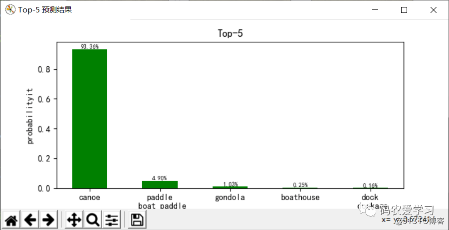
試験結果：

3.2結果分析

このボートの写真（/pic/8.jpg）をテストに使用します。プログラムは最初にトレーニングモデルパラメータファイル（vgg16.npy）をロードし、ネットワークパラメータ（重量バイアスなど）を辞書の形式で保存します。 、キー値を表示するために印刷できます。名前、ネットワークの順方向伝搬、画像入力は224x224x3です。ネットワーク層の数が増えると、データサイズは減少し続け、厚さは増加し続けます。 7x7x512になった後、1列のデータに引き伸ばされ、3つのレイヤーを通過します。完全に接続されたレイヤーとsoftmax分類出力により、最終モデルは、画像がカヌー（カヌー、カヌー）であるという93.36％の確実性でTop5予測結果を提供します。 、パドルボートパドル（パドルボート）であることが4.90％確実であり、予測効果は依然として良好です。

参照：人工知能の実践：Tensorflowノート