著者:chen_h
マイクロ・シグナル&QQ:862251340
マイクロチャネル公共数:coderpai
numpyのか、トーチで?
彼はトーチテンソル操作をスピードアップしますCPUのnumpyの配列として、(あなたが右のGPUを持っていることを提供する)のコンピューティング加速GPU上で生成することができますので、トーチは、numpyのニューラルネットワークコミュニティに主張しているため、ニューラルネットワーク場合もちろん、好ましくは、わずかにトーチテンソルデータの形式である。テンソルTensorflow同じ間等。
私たちは、彼はよくやったトーチとnumpyの互換性をnumpyのを形成するが、私たちのお気に入りのトーチを見るために使用されているので、もちろん、我々はまだ、numpyのが大好きです。たとえば、あなたが自由にnumpyの配列とトーチを変換することができますので、テンソルの:
import torch
import numpy as np

np_data = np.arange(6).reshape((2, 3))
torch_data = torch.from_numpy(np_data)
tensor2array = torch_data.numpy()
print(
    '\nnumpy array:', np_data,          # [[0 1 2], [3 4 5]]
    '\ntorch tensor:', torch_data,      #  0  1  2 \n 3  4  5    [torch.LongTensor of size 2x3]
    '\ntensor to array:', tensor2array, # [[0 1 2], [3 4 5]]
)
数学トーチで
実際には、テンソル操作とまったく同じトーチのnumpyの配列は、我々は、ビューの比較ポイントの形である。あなたが他の事業者に、より便利なトーチを学びたいのであれば、
# abs 绝对值计算
data = [-1, -2, 1, 2]
tensor = torch.FloatTensor(data)  # 转换成32位浮点 tensor
print(
    '\nabs',
    '\nnumpy: ', np.abs(data),          # [1 2 1 2]
    '\ntorch: ', torch.abs(tensor)      # [1 2 1 2]
)

# sin   三角函数 sin
print(
    '\nsin',
    '\nnumpy: ', np.sin(data),      # [-0.84147098 -0.90929743  0.84147098  0.90929743]
    '\ntorch: ', torch.sin(tensor)  # [-0.8415 -0.9093  0.8415  0.9093]
)

# mean  均值
print(
    '\nmean',
    '\nnumpy: ', np.mean(data),         # 0.0
    '\ntorch: ', torch.mean(tensor)     # 0.0
)
変数変数
トーチの変数は、ストアの場所は、値を変更しますです。内部の値は常に卵の数は変更していきます、ちょうど卵のロードされたバスケットのように、変化する。その中にその卵は誰なので、当然それはあります少しテンソルのトーチ。変数の同じタイプのリターンである変数の計算、もし。
私たちは、変数を定義します。
import torch
from torch.autograd import Variable # torch 中 Variable 模块

# 先生鸡蛋
tensor = torch.FloatTensor([[1,2],[3,4]])
# 把鸡蛋放到篮子里, requires_grad是参不参与误差反向传播, 要不要计算梯度
variable = Variable(tensor, requires_grad=True)

print(tensor)
"""
 1  2
 3  4
[torch.FloatTensor of size 2x2]
"""

print(variable)
"""
Variable containing:
 1  2
 3  4
[torch.FloatTensor of size 2x2]
"""
変数の計算勾配
私たちは、変数のテンソル計算と計算を比較します。
t_out = torch.mean(tensor*tensor)       # x^2
v_out = torch.mean(variable*variable)   # x^2
print(t_out)
print(v_out)    # 7.5
これまでのところ、我々は何も異なるが表示されていない、しかし、変数の計算は、それが計算グラフと呼ばれる静かにステップバイステップで、計算グラフの背後にある巨大な背景にシステムを設定するときは常に、覚えている。この図はやってするために使用されます?本来すべての時間算出ステップ(ノード)が互いに接続され、最終的に一度にすべての可変振幅変化(勾配)が計算される誤差逆方向伝送、およびテンソルは、この能力を持っていないであろう。
v_out = torch.mean(variable*variable) 計算に数字を追加するための計算ステップ、彼に信用は、私たちはあなたに例をあげる復路がある計算誤差は次のようになります。
v_out.backward()    # 模拟 v_out 的误差反向传递

# 下面两步看不懂没关系, 只要知道 Variable 是计算图的一部分, 可以用来传递误差就好.
# v_out = 1/4 * sum(variable*variable) 这是计算图中的 v_out 计算步骤
# 针对于 v_out 的梯度就是, d(v_out)/d(variable) = 1/4*2*variable = variable/2

print(variable.grad)    # 初始 Variable 的梯度
'''
 0.5000  1.0000
 1.5000  2.0000
'''
バリアブルデータは内部の取得します
直接print(variable)多くの場合(例えば、PLTと描きたい)を取るされていないデータの可変形式、出力のみ、我々はそれを変換する必要がありますので、それはテンソルの形になります。
print(variable)     #  Variable 形式
"""
Variable containing:
 1  2
 3  4
[torch.FloatTensor of size 2x2]
"""

print(variable.data)    # tensor 形式
"""
 1  2
 3  4
[torch.FloatTensor of size 2x2]
"""

print(variable.data.numpy())    # numpy 形式
"""
[[ 1.  2.]
 [ 3.  4.]]
"""
トーチ活性化関数
トーチ機能は、モチベーションをたくさん持っているが、我々は通常、わずか数を使用しています。relu、sigmoid、tanh、softplus。その後、我々は、彼らが彼らの友人のように見えるものを参照してください。
import torch
import torch.nn.functional as F     # 激励函数都在这
from torch.autograd import Variable

# 做一些假数据来观看图像
x = torch.linspace(-5, 5, 200)  # x data (tensor), shape=(100, 1)
x = Variable(x)
次の世代は、励起の異なる機能のデータを行うことです。
x_np = x.data.numpy()   # 换成 numpy array, 出图时用

# 几种常用的 激励函数
y_relu = F.relu(x).data.numpy()
y_sigmoid = F.sigmoid(x).data.numpy()
y_tanh = F.tanh(x).data.numpy()
y_softplus = F.softplus(x).data.numpy()
# y_softmax = F.softmax(x)  softmax 比较特殊, 不能直接显示, 不过他是关于概率的, 用于分类
その後、我々はコードを描き、描画を開始以下のとおりです。
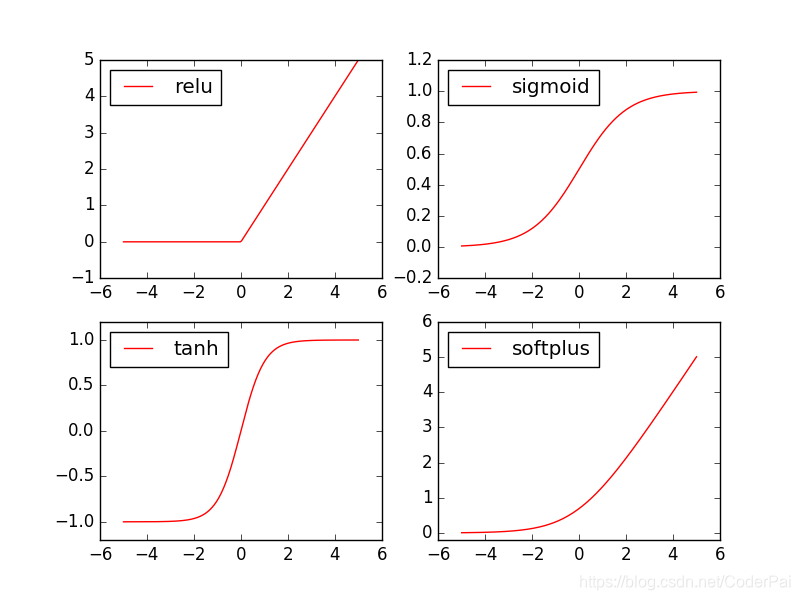
import matplotlib.pyplot as plt  # python 的可视化模块, 我有教程 (https://morvanzhou.github.io/tutorials/data-manipulation/plt/)

plt.figure(1, figsize=(8, 6))
plt.subplot(221)
plt.plot(x_np, y_relu, c='red', label='relu')
plt.ylim((-1, 5))
plt.legend(loc='best')

plt.subplot(222)
plt.plot(x_np, y_sigmoid, c='red', label='sigmoid')
plt.ylim((-0.2, 1.2))
plt.legend(loc='best')

plt.subplot(223)
plt.plot(x_np, y_tanh, c='red', label='tanh')
plt.ylim((-1.2, 1.2))
plt.legend(loc='best')

plt.subplot(224)
plt.plot(x_np, y_softplus, c='red', label='softplus')
plt.ylim((-0.2, 6))
plt.legend(loc='best')

plt.show()
リンク:
https://morvanzhou.github.io/tutorials/machine-learning/torch/
https://pytorch.org/docs/stable/torch.html
https://pytorch.org/docs/stable/torch.html
