Python Practical Technology 2: Data Analysis and Visualization (2)

➢Multidimensional array library, it is very convenient to create multidimensional arrays and can replace multidimensional lists
➢It is faster than multidimensional lists
➢Supports various mathematical operations of vectors and matrices
➢All element types must be the same

1. Operation function:

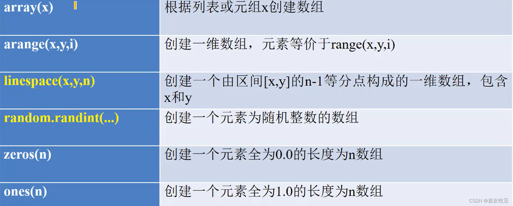
import numpy as np    #以后numpy简写为np
print (np.array([1,2,3]) )    #>>[1 2 3]
print (np. arange(1,9,2) )    #>>[13 5 7]
print (np. linspace(1,10,4))    #>>[ 1.  4.   7.   10. ]
print (np . random. randint (10,20, [2,3]) )    
#>>[[12 19 12]
#>> [19 13 10 ]]

print (np . random. randint (10,20,5) ) #>> [12 19 19 10 13]
a = np. zeros (3)
print (a)
#>>[ 0. 0. 0.]

print(list(a) )
#>>[0.0，0.0，0.0]

a = np. zeros((2 ,3) ,dtype=int) #创建- t个2行3列的元素都是整数0的数组

import numpy as np
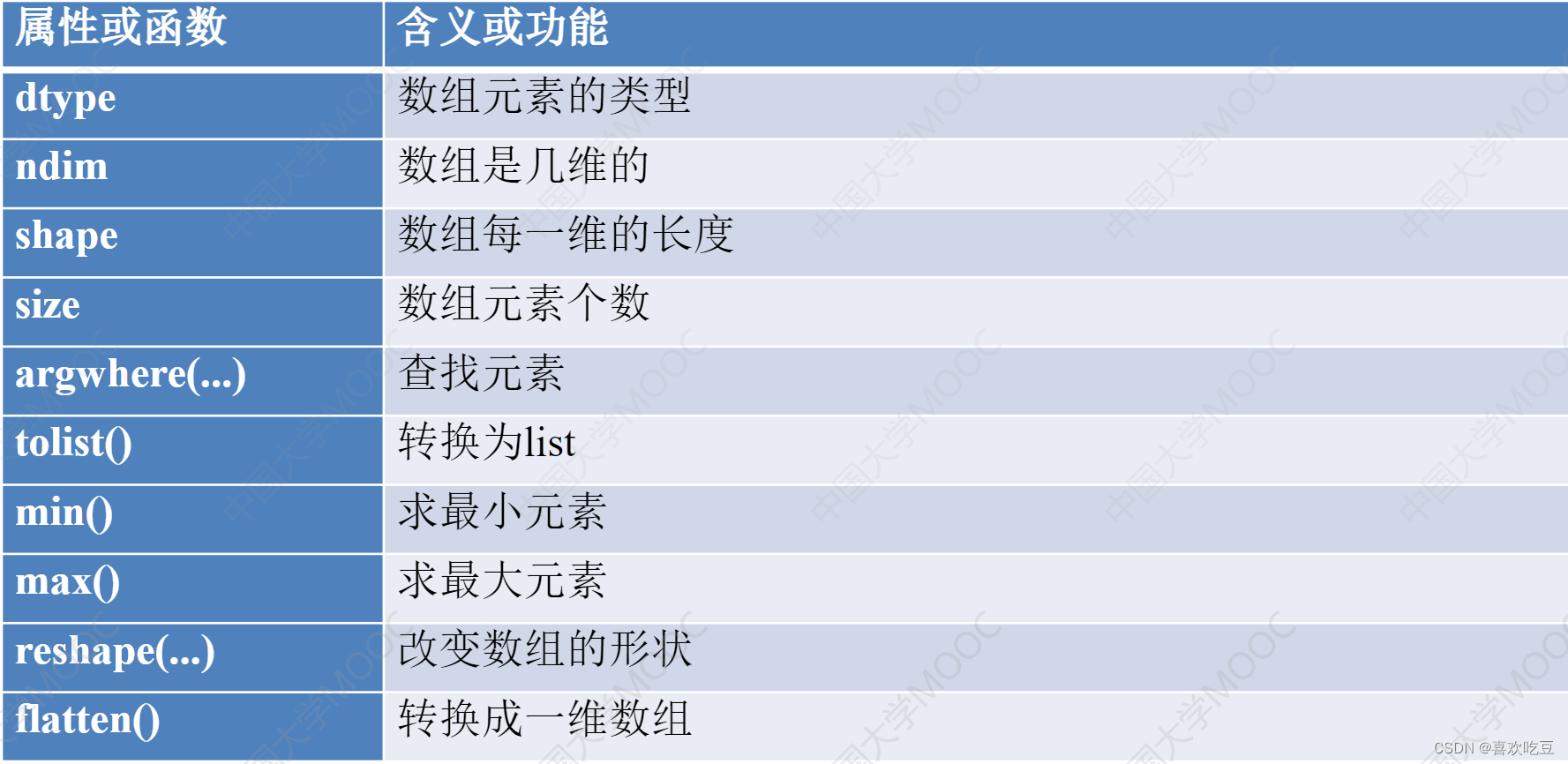
b = np.array([i for i in range (12) ])
#b是[ 0 1 5 6 7 8 9 10 11]
a = b.reshape( (3,4) )
#转换成3行4列的数组，b不变

print (len(a) )
#>>3   a有3行

print(a. size )
#>>12   a的元素个数是12
print (a. ndim)
#>>2   a是2维的

print (a. shape)
#>>(3, 4)   a是3行4列

print (a. dtype)
#>>int32 a的元素类型 是32位的整数
L = a.tolist ()
#转换成列表，a不变

print (L)
#>>[[0，1，2，3]，[4,5，6，7]，[8，9，10，11]]
b = a. flatten ()
#转换成一维数组

print (b)
#>>[0 1 2 3 5 6 7 8 9 10 11]

2. Add and delete numpy array elements

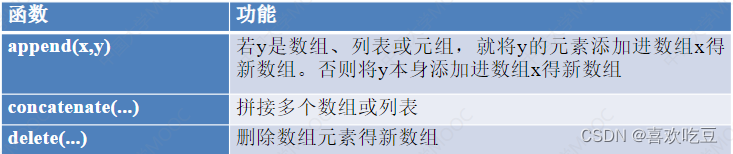
Once a numpy array is generated, elements cannot be added or deleted. The above function returns a new array.

1) Add array elements

import numpy as np
a = np.array((1,2,3) )
#a是[123]

b = np. append(a,10)<
#a不会发生变化
print (b)
#>>[1 2 3 10]

print (np. append(a, [10,20] ) )
#>>[1 2 3 10 20]

C=np. zeros ( (2,3) , dtype=int)
#c是2行3列的全0数组

print (np. append(a,c) )
#>>[1 2 3 0 0 0 0 0 0]

print (np. concatenate( (a, [10,20] ,a)) )
#>>[1 2 3 10 20 1 2 3]

print (np. concatenate( (C, np. array([[10 ,20,30]] ) ) ) )
#c拼接一行[10, 20 ,30]得新数组

print (np. concatenate( (C, np.array([[1,2], [10,20]])) ,axis=1) )
#c的第0行拼接了1，2两个元素、第1行拼接了10 , 20两个新元素后得到新数组

2) numpy deletes array elements

import numpy as np
a = np.array((1,2,3,4) )
b = np.delete(a,1) #删除a中下标为1的元素, a不会改变
print (b)
#>>[1_ 3 4]

b = np.array([[1,2,3,4] ,[5,6, 7,8], [9,10,11,121])
print (np. delete (b,1 ,axis=0) )
#删除b的第1行得新数组
#>>[[1 2 3 4]
#>>[9 10 11 12]]

print (np. delete (b,1 ,axis=1) )
#删除b的第1列得新数组

print (np. delete (b,[1,2] ,axis=0) )
#删除b的第1行和第2行得新数组

print (np. delete (b,[1,3] ,axis=1) )
#删除b的第1列和第3列得新数组

3) Find elements in numpy array

import numpy as np
a = np.array( (1,2,3,5,3,4) )
pos = np. argwhere(a==3)
#pos是[[2] [4] ]

a = np.array([[1,2,3] , [4,5,2]])
print(2 in a)
#>>True

pos = np. argwhere(a==2)
#pos是[[0 1] [1 2]]

b = a[a>2]
#抽取a中大于2的元素形成一个一维数组

print (b)
#>>[3 4 5]

a[a>2]=-1
#a变成[[12-1][-1-12]]

4) Mathematical operations on numpy arrays

import numpy as np
a = np.array( (1,2,3,4) )
b=a+1
print (b)
#>>[2 3 4 5]

print (a*b)
#>>[2 6 12 20]    a,b对应元素相乘
print (a+b)
#>>[3579]a,b对应元素相加

c = np.sqrt(a*10)     #a*10是[10 20 30 40]

print(c) 
#>>[ 3. 16227766 4. 47213595 5. 47722558 6.32455532]

3. Slice of numpy array

A slice of a numpy array is a "view", which is a part of the original array, not a copy of a part.

import numpy as np
a=np.arange(8)
#a是[0 1 2 3 4 5 6 7]

b = a[3:6]
#注意，b是a的一部分

print (b)
#>>[3 4 5]

c = np.copy(a[3:6])
#c是a的一部分的拷贝

b[0] = 100
#会修改a

print(a)
#>>[ 0 1 2 100 4 6 7]

print(c)
#>>[3 4 5] c不受b影响

a = np.array([[1,2,3,4] ,[5,6,7,8] , [9,10,11,12] , [13,14,15,16]])
b = a[1:3,1:4]
#b是>>[[678][101112]]

2. Data analysis library pandas

1. DataFrame construction and access

➢The core function is to perform various operations on two-dimensional tables, such as adding, deleting, modifying, and finding the sum, variance, median, average, etc. of column data. ➢Requires numpy support. ➢If there is openpyxI or xIrd or xIwt
support
, You can also read and write excel documents.
➢The most critical class: DataFrame, representing a two-dimensional table

Important classes of pandas: Series

Series is a one-dimensional table. Each element is labeled and subscripted. It has both list and dictionary access forms.

import pandas as pd
s = pd. Series (data=[80, 90,100] , index=['语文', '数学', '英语'])
for x in s:
#>>80 90 100 

print(x,end=" ")
print ("")
print(s['语文'] ,s[1])
#>>80 90    标签和序号都可以作为下标来访问元
print(s[0:2] [ '数学'])
#>>90    s[0:2]是切片
print(s['数学': '英语'] [1])
#>>100

for i in range (len (s. index) ) :
#>>语文 数学 英语

print(s. index[i] ,end = " ")
s['体育'] = 110
#在尾部添加元素，标签为'体育'，值为110

s. pop('数学')
#删除标签为'数学’的元素

s2 = s. append (pd . Series (120, index = [' 政治'])) #不改变s
print(s2['语文'] ,s2['政治'])
#>>80 120

print (1ist(s2) )
#>>[80，100， 110， 120]

print(s.sum() ,s.min() ,s .mean() ,s . median() )
#>>290 80 96. 66666666667 100.0输出和、 最小值、平均值、中位数>

print (s . idxmax() ,s. argmax () )
#>>体育 2    输出最大元素的标签和下标

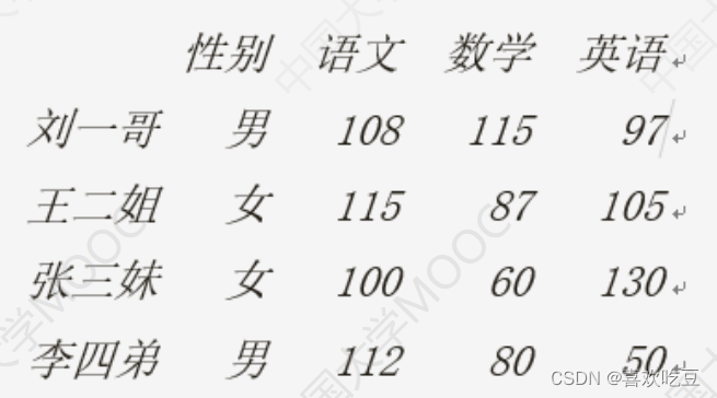
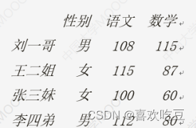
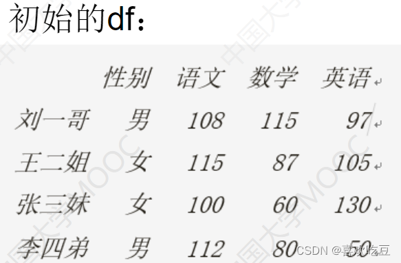
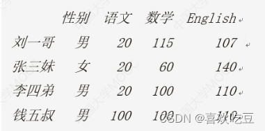
DataFrame is a two-dimensional table with row and column labels, each column is a Series

import pandas as pd
pd.set_ option( 'display . unicode.east asian width' , True)
#输出对齐方面的设置

scores = [['男' ,108 ,115,97] ,['女' ,115,87,105] , ['女' ,100, 60 ,130]
['男' ,112,80,50]]
names = ['刘一哥，'王二姐’，'张三妹'，李四弟'] .
courses = ['性别', '语文', '数学', '英语']
df = . pd.DataFrame (data=scores ,index = names , columns = courses)
print (df)

print (df. values[0] [1] , type (df. values) ) #>>108. <class numpy . ndarray '>
print (list (df. index) )
#>>['刘一哥'，'王二姐'，'张三妹'，'李四弟']

print (list (df. columns) )
#>>['性别'，'语文'，'数学'，'英语']

print (df . index[2] ,df . columns[2]) #>>张三妹 数学
s1 = df['语文']
#s1是个Series,代表'语文'那一列

print(s1['刘一哥'] ,s1[0])
#>>108 108    刘一哥语文成绩
print(df['语文']['刘一哥'])
#>>108    列索引先写
s2 = df.1oc['王二姐']
#s2也是个Series,代表“王二姐”那一行

print(s2['性别'] ,s2['语文'] ,s2[2])
#>>女 115 87     二姐的性别、语文和数学分数

2. DataFrame slicing and statistics

#DataFrame的切片：
#1loc[行选择器,.列选择器]    用下标做切片
#Ioc[行选择器，列选择器]    用标签做切片
#DataFrame的切片是视图

df2 = df. iloc[1:3]    #行切片，是视图，选1 ,2两行
dt2 = df.1c['王二姐':张三妹']    #和上一行等价
print (df2)

df2 = df. i1oc[: ,0:3]    #列切片(是视图)，选0、1. 2三列
df2 = df.1oc[:, '性别': '数学']     #和上一行等价
print (df2)

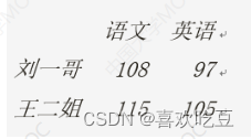
df2 = df.i1oc[:2,[1,3]]    #行列切片
df2 = df.1oc[:'王二姐'，['语文', '英语']]    #和上一行等价
print (df2)

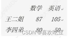
df2 = df.i1oc[[1,3] ,2:4]    #取第1、3行,第2、3列<
df2 = df.1oc[['王二姐' , '李四弟']，'数学': '英语']     #和上一行等价
print (df2)

3. DataFrame analysis statistics

print ("---下面是DataFrame的分析和统计---")
print (df. T)
#df . T是df的转置矩阵,即行列互换的矩阵

print (df . sort_ values ( '语文' , ascending=False)) #按语文成绩降序排列
print (df.sum() [ '语文'] ,df .mean() ['数学'],df .median() ['英语'])
#>>435 85.5 101.0语文分数之和、 数学平均分、英语中位数

print(df .min() ['语文'] ,df .max() ['数学'])
#>>100 115   语文最低分，数学最高分
print (df .max(axis = 1)['王二姐'1) #>>115 二姐的最高分科目的分数
print (df['语文' ] . idxmax() )
#>>王二姐  语文最高分所在行的标签
print(df['数学] . argmin())
#>>2  数学最低分所在行的行号
print (df.1oc[ (df['语文'] > 100) & (df['数学'] >= 85)])

4. Modification, addition and deletion of DataFrame

print ("---下面是DataFrame的增删和修改---")
df.1oc['王二姐', '英语'] = df. iloc[0,1] = 150     #修改王二姐英语和刘一哥语文成绩
df['物理'] = [80, 70,90,100]
#为所有人添加物理成绩这-列

df. insert(1, "体育", [89,77, 76,45])
#为所有人插入体育成绩到第1列

df.1oc['李四弟'] = ['男' ,100 ,100 ,100 ,100,100]     #修改李四弟全部信息
df.1oc[: , '语文'] = [20,20,20,20]
#修改所有人语文成绩

df.1oc[ '钱五叔'] = [ '男' , 100 , 100 ,100, 100 , 100]
#加一行

df.1oc[: , '英语'] += 10
#>>所有人英语加10分

df. columns = ['性别', '体育', '语文', '数学', 'English', '物理'] #改列标签
print (df)

df.drop( ['体育', '物理'] ,axis=1, inplace=True) #删除体育和物理成绩
df.drop( '王二姐' ,axis = 0，inplace=True)
#删除王二姐那一行

print (df)

df.drop ( [df. index[i] for i in range(1,3) ] ,axis=0 , inplace = True)
#删除第1,2行
df .drop( [df . columns[i] for i in range(3) ] ,axis = y 1 , inplace=
True) #删除第0到2列

5. Read and write excel and csv documents

➢Requires openpyxI (for .xIsx files) or xIrd or xIwt support (old .xls files)
➢Each worksheet read is a DataFrame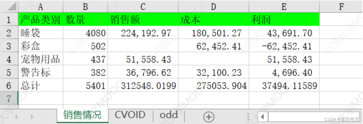

1) Use pandas to read excel documents

import pandas as pd
pd.set option ( ' display . unicode.east asian width' , True)
dt = pd. read excel ("'excel sample.xlsx" , sheet name= [ '销售情况' ,1] ,
index col=0) #读取第0和第1张二工作表
df =
dt [ '销售情况']
#dt是字典，df是DataFrame

print (df. iloc[0,0] ,df.loc[ 'I睡袋' , '数量'])
#>>4080 4080

print (df)

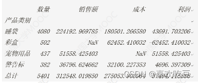
print (pd. isnu1l (df.1oc['彩盒', '销售额']))
#>> True
df . fillna (0 , inplace= =True)
#将所有NaNa用0替换
print(df.loc[ '彩盒' , '销售额'] ,df. iloc[2,2] )
#>>0.0 0.0

df.to excel (filename, sheet_ name="Sheet1", na_ rep='',.. ...)
➢Write the data in the DataFrame object df to the "Sheet1" worksheet in the exce1 document filename, NaN is replaced with ' '.
➢The original filename file will be overwritten
➢If you want to write multiple worksheets in an excel document, you need to use ExcelWrite

# (接.上面程序)

writer = pd. Exce 1Writer ("new.x1sx")
#创建ExcelWri ter对象

df. to exce1 (writer , sheet_ name="S1")
df.T. to exce1 (writer, sheet_ name="S2")
#转置矩阵写入

df.sort_ values( '销售额' , ascending= False) . to exce1 (writer ,
sheet_ name="S3")
#按销售额排序的新DataFrame写入工作表s3

df[ '销售额'] . to excel (writer ,sheet_ name="S4")
#只写入一列
writer . save ()

2) Use pandas to read and write csv files

df. to_ csv (" result. csv" ,sep=" ," ,na rep= 'NA' ,
float_ format="号 .2f" , encoding="gbk")

df = pd. read csv (" result. csv")

3. Use matplotlib for data display

1. Draw a histogram

import matp1otlib. pYp1ot as plt     #以后plt等价于ma tplotlib . pyplot
from ma tp1ot1ib import rcParams
rcParams[ ' font. family'] = rcParams[ ' font. sans-serif'] = ' SimHei '
#设置中文支持,中文字体为简体黑体

ax = p1t. figure() .add subp1ot ()
#建图，获取子图对象ax

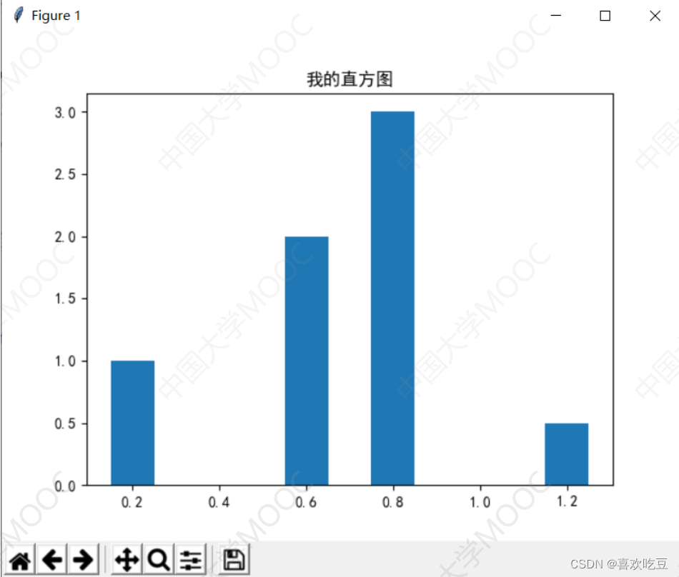
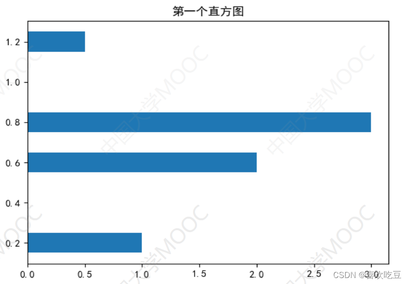
ax.bar(x = (0.2,0.6,0.8,1.2) ,height = (1,2,3,0.5) ，width = 0.1)
#x表示4个柱子中心横坐标分别是0.2,0.6,0.8,1
#height表示4个柱子高度分别是1,2,3,0.5
#width表示柱子宽度0.1

ax.set_ title ('我的直方图)
#设置标题

p1t. show ()
#显示绘图结果

纵向
ax.bar(x = (0.2,0.6,0.8,1.2) ,height = (1,2,3,0.5) ,width = 0.1)
横向
ax.barh(y = (0.2,0.6,0.8,1.2) ,width = (1,2,3,0.5) ，height = 0.1)

2. Draw a stacked histogram

import ma tplotlib. pyp1ot as p1t
ax = plt. figure() . add subp1ot()
labels = ['Jan' ，'Feb' ，'Mar' ，lApr']
num1 = [20， 30， 15， 35]
#Dept1的数据

num2 = [15， 30，40， 20]
#Dept2的数据

cordx = range (len (num1) )
#x轴刻度位置

rects1 = ax.bar(x = cordx，height=num1, width=0.5， color=' red' ,
label="Dept1")
rects2 = ax.bar(x = cordx， height=num2， width=0 .5，color='green' ,
label="Dept2"，bottom= =num1 )

ax.set_ y1im(0， 100) 
#y轴坐标范围
ax. set_ ylabel ("Profit")
#y轴含义(标签) 
ax. set xticks (cordx )
#设置x轴刻度位置
ax. set_ xlabel ("In year 2020")
#x轴含义(标签)

ax.set_ title ("My Company")
ax. legend()
#在右上角显示图例说明

p1t. show ()

3. Draw a comparison histogram (with multiple sets of data)

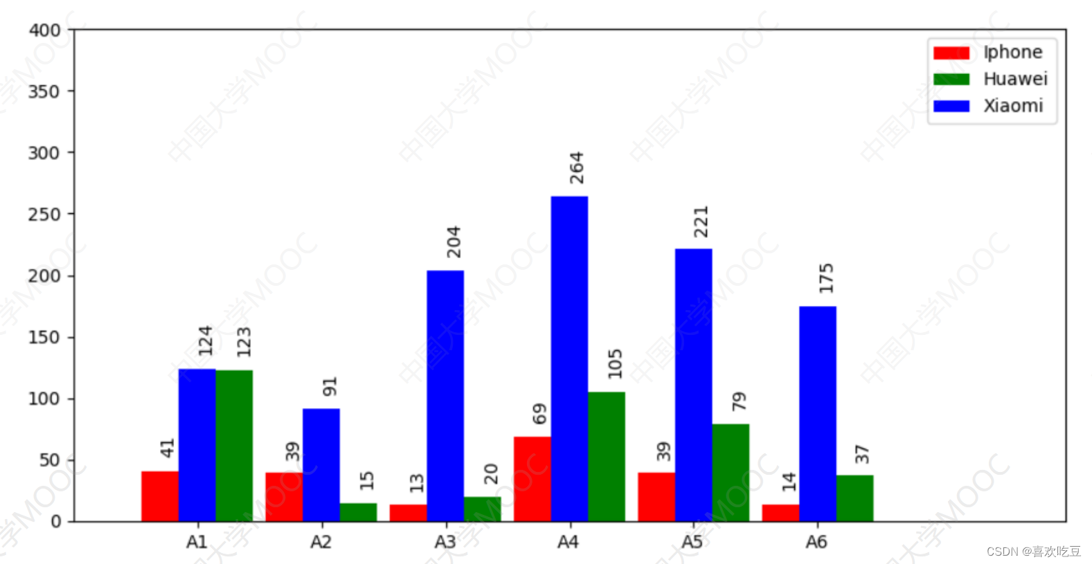
import matplotlib. pyp1ot as plt
ax =. plt. figure (figsize= (10,5)) . add_ subplot ()     #建图，获取子图对象ax
ax.set ylim(0, 400)
#指定y轴坐标范围

ax.set xlim(0, 80)
#指定x轴坐标范围
#以下是3组直方图的数据

x1=[7，17，27，37，47，57]
#第一-组直方图每个柱子中心点的横坐标
x2 = [13， 23，33，43， 53，63] #第二组直方图每个柱子中心点的横坐标
x3 = [10， 20，30，40， 50， 60]

y1 = [41， 39，13，69，39， 14]
#第一组直方图每个柱子的高度
y2 = [123，15, 20，105，79，37] #第二组直方图每个柱子的高度
y3 = [124，91， 204， 264，221, 175]

rects1 = ax.bar(x1， y1，facecolor='red' ，width=3， label =_ ' Iphone' )
rects2 = ax.bar (x2，y2，facecolor='green' ，width=3， label = ' Huawei ' )
rects3 = ax.bar(x3， y3，facecolor= ='blue'，width=3，label = ' Xiaomi )

ax.set_ xticks (x3)
#x轴在x3中的各坐标点下面加刻度

ax. set_ xticklabels( ('A1', 'A2', 'A3', 'A4' , 'A5', 'A6') )
#指定x轴上每- -刻度下方的文字

ax. legend ()
#显示右.上角三组图的说明

def 1abe1 (ax , rects) :    #在rects的每个柱子顶端标注数值
for rect in rects :
height = rect.get_ height()
ax. text (rect.get_ x() + rect.get_ width() /2,
height+14, str (height) , rotation=90) #文字旋转90度
1abe1 (ax, rects1)
label (ax , rects2)
labe1 (ax, rects3)
p1t. show ()

4. Draw scatter points and line charts

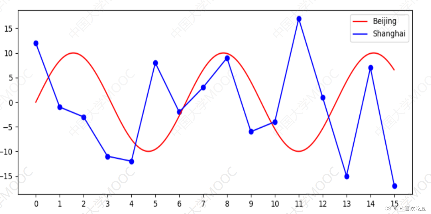
import math , random
import matplotlib.pyplot as plt
def drawPlot(ax) :
xs = [i / 100 for i in range (1500)] #1500个 点的横坐标，间隔0 .01
ys = [10*math.sin(x) for X in xs]
#对应曲线y=10*sin (x).上的1 500个点的y坐标

ax.plot (xs,ys, "red" ,label = "Beijing") #画曲线y= =10*sin (x)
ys = list (range(-18,18) )
random. shuffle (ys)

ax. scatter (range(16)，ys[:16] ，c = "blue") #画散点
ax.plot (range(16)，ys[:16] ，"blue", label=" Shanghai") #画折线

ax . legend ()
#显示右.上角的各条折线说明

ax.set xticks (range (16) )
#x轴在坐标0,1.. .15处加刻度
ax. set_ xticklabels (range (16)) #指定x轴每个刻度 下方显示的文字

ax = plt. figure (figsize=(10，4) ,dpi=100) .add_ subp1ot() #图像长宽和清晰度
drawP1ot (ax)
p1t. show ()

5. Draw a pie chart

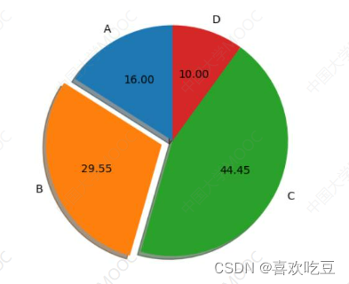
import matplotlib.pyplot as p1t .
def drawPie (ax) :
1bs = ( 'A','B', 'C',
'D' )
#四个扇区的标签
sectors = [16， 29.55， 44.45， 10]
#四个扇区的份额(百分比)
exp1 = [0， 0.1, 0，0]
#四个扇区的突出程度
ax.pie (x=sectors，labels=lbs， exp1ode=exp1,
autopct=18.2f' , shadow=True, labeldistance=1 .1,
pctdistance = 0 .6, startangle = 90)

ax.set_ title ("pie sample")
#饼图标题

ax = p1t. figure() .add subp1ot()
drawPie (ax)
p1t. show()

6. Draw a heat map

import numpy as np
from matplotlib import pyp1ot as plt
data = np. random. randint(0，100， 30) .reshape (5，6)
#生成一一个5行六列，元素[0, 100]内的随机矩阵
xlabels = [ 'Beijing', ' Shanghai'，'Chengdu' ,
' Guangzhou'，' Hangzhou'，
' Wuhan' ]
ylabels=['2016'，'2017'，'2018'，'2019'，'20201]
ax = plt. figure (figsize=(10,8)) .add_ subp1ot()
ax.set yticks (range (len (ylabels))) #y轴在坐标 [0 , len (ylabels))处加刻度
ax.set_ yticklabels (ylabels) #设置y轴刻度文字

ax. set_ xticks (range (len (xlabels) ) )
ax.set xticklabels (xlabels)
heatMp = ax. imshow (data，cmap=plt. cm.hot, aspect=' auto' ,
vmin =0,vmax=100)

for i in range (1en (x1abe1s) ) :
for j in range (1en (y1abe1s) ) :
ax. text(i,j ,data[j] [i] ,ha = "center" ,va = "center"
color =
"blue" ,size=26)
p1t. colorbar (heatMp)
#绘制右边的颜色-数值对照柱
plt . xticks (rotation=45 , ha=" right") #将x轴刻度文字进行旋转, 且水平方向右对齐
p1t. title ("Sales Volume (ton) ")
p1t. show ()

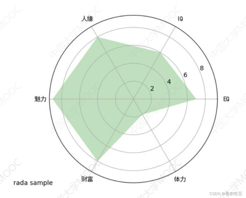
7. Draw a radar chart

import matplotlib. pyplot as plt
from matplotlib import rcParams
#处理汉字用

def drawRadar (ax) :
pi = 3.1415926
labels = ['EQ', 'IQ','人缘' , '魅力', '财富' , '体力'] #6个属性的名称
attrNum = len (labels)
#attrNum是属性种类数，处等于6
data = [7 ,6,8,9,8,2]
#六个属性的值
angles = [2*pi *i/ attrNum  for i in range (attrNum) ]
#angles是以弧度为单位的6个属性对应的6条半径线的角度
angles2 = [x * 180/pi for x in angles]
#angles2是以角度为单位的6个属性对应的半径线的角度
ax.set ylim(0，10)
#限定半径线上的坐标范围

ax. set_ thetagrids (angles2，labels , fontproperties="SimHei" )
#绘制6个属性对应的6条半径

ax. fi1l (angles，data, facecolor= ; : 6 'g' ,alpha= =0.25)
#填充，alpha :透明度

rcParams[' font. family'] = rcParams[' font. sans-serif'] = ' SimHei '
#处理汉字
ax = p1t. figure() . add_ subplot (projection = "polar")
#生成极坐标形式子图
drawRadar (ax)
p1t. show ()

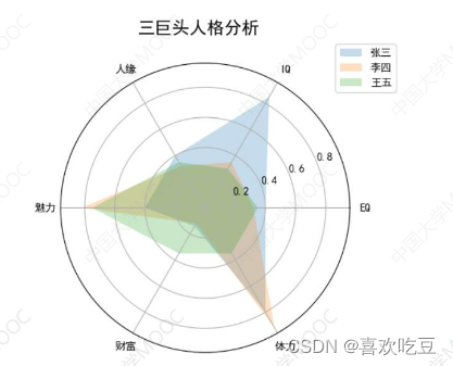
8. Draw multi-layer radar charts

import matplotlib.pyplot as p1t
from ma tplot1ib import rcPar ams
rcParams[ ' font. family'] = rcParams[ ' font. sans-serif'] = ' SimHei !
pi = 3.1415926
labels = ['EQ', 'IQ','人缘', '魅力',财富', '体力] #6个属性的名称
attrNum = len (labels)
names = (张三',李四'王五
data = [[0.40,0.32,0.35] ，
[0.85,0.35,0.30] ,
[0.40,0.32,0.35]，[0.40,0.82,0.75] ,
[0.14,0.12,0.35] ,
[0.80,0.92,0.35]]
#三个人的数据

angles = [2*pi*i/attrNum for i in range (attrNum) ]
angles2 = [x * 180/pi for x in ang1es]
ax = p1t. figure() .add_ subp1ot (projection = "polar")

ax. set_ the tagrids (angles2 , labels)
ax.set_ title('三巨头人格分析',y = 1.05) #y指明标题垂直位置
ax. legend (names , 1oc=(0.95,0.9)) #画出右上角不同人的颜色说明
plt. show ()

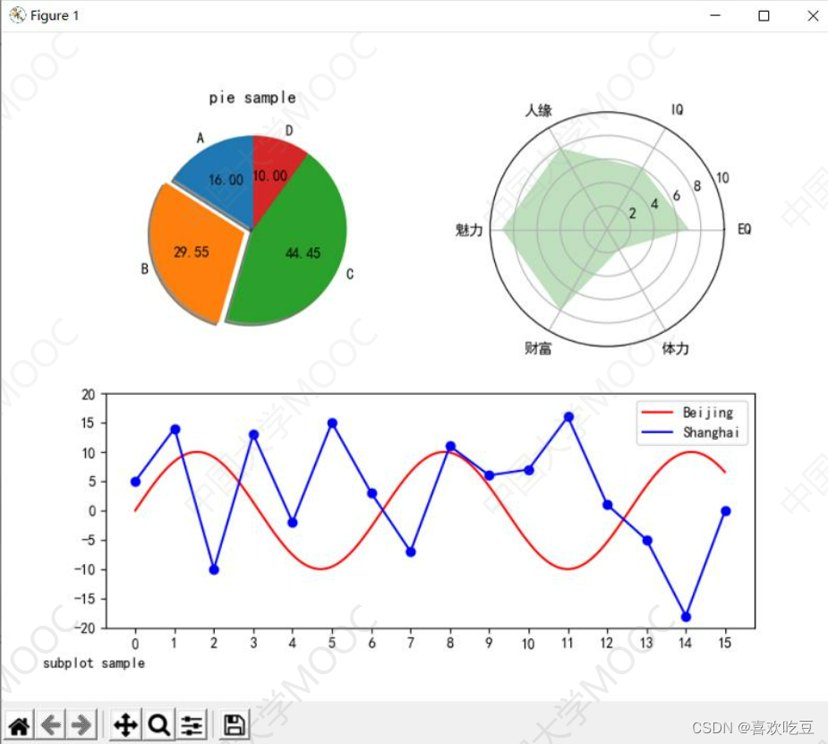
9. Draw multiple subgraphs

#程序中的import、汉字处理及drawRadar、 drawPie、 drawPlot函数略， 见前面程序
fig = plt. figure (figsize=(8,8) )
ax = fig.add subplot(2,2,1) #窗口分割成2*2,取位于第1个方格的子图
drawPie (ax)
ax = fig.add subplot(2 ,2 ,2 ,projection = "polar" )
drawRadar (ax)
ax = p1t. subp1ot2grid( (2, 2)，(1， 0)，colspan=2)
#或写成: ax = fig.add subplot(2,1,2)

drawPlot (ax)
plt. figtext(0.05,0.05, ' subplot sample' )
#显示左下角的图像标题

plt. show ()