Based on random forest + small intelligent health recommendation assistant (heart disease + chronic kidney disease health prediction + drug recommendation) - machine learning algorithm application (including Python engineering source code) + data set (1)

---

Preface

This project is based on publicly available data sets on Kaggle and aims to conduct in-depth feature screening and extraction of heart disease and chronic kidney disease. It utilizes a random forest machine learning model that is trained on these features to predict whether one has these diseases. Not only that, the project will also provide relevant drug recommendations based on the patient's symptoms or needs, thus realizing a highly practical intelligent medical assistant.

First, the project collected public data sets from Kaggle, which contain rich information related to heart disease and chronic kidney disease. Then, through data preprocessing and feature engineering, the most relevant features are extracted from these data for training of machine learning models.

Next, the project employed a random forest machine learning model, a powerful classification algorithm. By using training data, the model is able to learn how different features are associated with heart disease and chronic kidney disease. Once the model is trained, it can make predictions on new patient data to determine whether the patient has these diseases.

In addition to disease prediction, the project also features a drug recommendation system. Based on the patient's symptoms, needs and disease diagnosis, the system will recommend appropriate medications and treatment options to provide more comprehensive medical support.

Taken together, this project can not only predict heart disease and chronic kidney disease, but also provide personalized treatment recommendations. This kind of intelligent medical assistant is expected to improve the accuracy of medical decision-making, provide patients with a better medical experience, and play a positive role in the reasonable allocation of medical resources.

overall design

This part includes the overall system structure diagram and system flow chart.

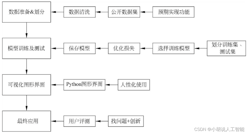
Overall system structure diagram

The overall structure of the system is shown in the figure.

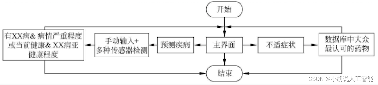
System flow chart

The system flow is shown in the figure.

Operating environment

Python environment

Python 3.6 and above configuration is required. In Windows environment, it is recommended to download Anaconda to complete the configuration of the environment required for Python. The download address is https://www.anaconda.com/ . You can also download a virtual machine to run the code in Linux environment.

Dependent libraries

Use the following command to install:

pip install pandas

Module implementation

This project includes 2 functions, each function has 3 modules: disease prediction, drug recommendation, and module application. The function introduction and related codes of each module are given below.

1. Disease prediction

This module is a small health prediction system that predicts two diseases: heart disease and chronic kidney disease.

1) Data preprocessing

The source address of the heart disease data set is https://archive.ics.uci.edu/dataset/45/heart+disease ; the source address of the chronic kidney disease data set is https://www.kaggle.com/mansoordaku/ckdisease . Both data sets include age, gender, resting blood pressure, cholesterol levels and other data of more than 300 test subjects.

Heart disease data set preprocessing

Loading data sets and data preprocessing are mostly implemented through the Pandas library. The relevant code is as follows:

#导入相应库函数
import pandas as pd
#读取心脏病数据集
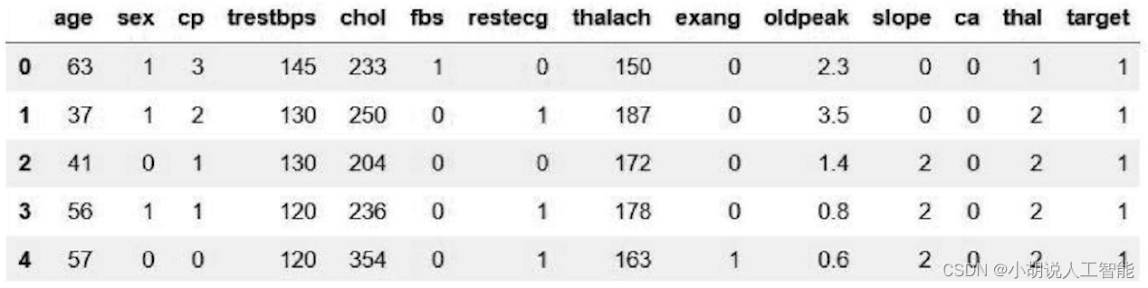
df = pd.read_csv("../Thursday9 10 11/heart.csv")
df.head()

Automatically read the corresponding data from csv, as shown in the figure.

Check whether the data has a default value. If there is data, it will be displayed as NaN. When the data has a default value, the data plot cannot be visualized.

#检查是否有缺省值
df.loc[(df['age'].isnull()) |
       (df['sex'].isnull()) |
       (df['cp'].isnull()) |
       (df['trestbps'].isnull()) |
       (df['chol'].isnull()) |
       (df['fbs'].isnull()) |
       (df['restecg'].isnull()) |
       (df['thalach'].isnull()) |
       (df['exang'].isnull()) |
       (df['oldpeak'].isnull()) |
       (df['slope'].isnull()) |
       (df['ca'].isnull()) |
       (df['target'].isnull())]

There is no default value in the data set, and the scale of the data is relatively large. Error data can be checked through drawing observation, as shown in the figure.

#通过seaborn绘图,观察数据
sns.pairplot(df.dropna(), hue='target')

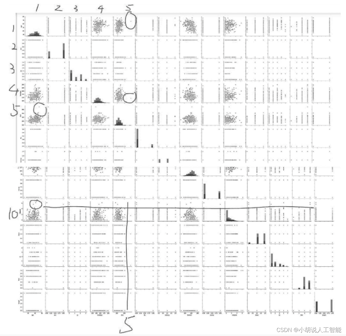
Through observation, some points in the fifth column (blood cholesterol content) and the tenth row (resting blood pressure) are far away from other points. Draw a data distribution chart for further analysis.

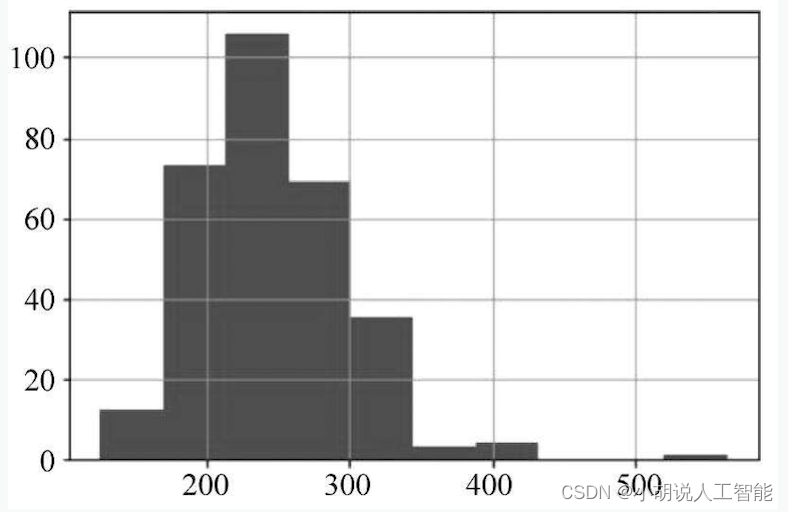
#绘制血液中胆固醇数据分布
df['chol'].hist()
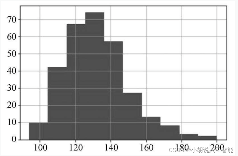
#绘制静息血压分布图
df[‘treatbps’].hist()

The data distribution is shown in Figures 1 and 2. The cholesterol content in the blood reaches 500, and the maximum resting blood pressure reaches 200. After reviewing the data, the normal value of resting blood pressure should be between 120 and 140, but the patient data close to 200 is realistic. It was also the patient who obtained the maximum cholesterol level, and there was no data that was inconsistent with the actual situation.

Figure 1 Cholesterol content in blood

Figure 2 Resting blood pressure

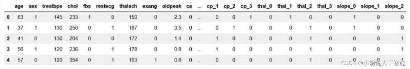
The following is to change the data type. For example, chest pain type, 1 to 4 are categorical variables. Its size is not comparative, but the numerical size will affect the weight during training. Therefore, we need to convert categorical variables into dummy variables, split the 4 categories into 4 pieces, and use 0 and 1 to represent yes or no respectively.

#将类别变量转换为伪变量
a = pd.get_dummies(df['cp'], prefix = "cp")
b = pd.get_dummies(df['thal'], prefix = "thal")
c = pd.get_dummies(df['slope'], prefix = "slope")
frames = [df, a, b, c]
df = pd.concat(frames, axis = 1)
#保留转换后的变量即可，删除原来的类别变量
df = df.drop(columns = ['cp', 'thal', 'slope'])

As shown in the figure after successful conversion.

Finally, Scikit-learn is used to train_test_split()automatically divide the training set and test set.

#标签是target，是否患病
y = df.target.values
x_data = df.drop(['target'], axis = 1)  
#丢弃标签，也就是最后一行target
#按4:1划分训练集测试集
x_train, x_test, y_train, y_test = train_test_split(x_data,y,test_size = 0.2,random_state=0)
x_train = x_train.T
y_train = y_train.T
x_test = x_test.T
y_test = y_test.T
#心脏病数据集预处理完成

Chronic kidney disease data preprocessing

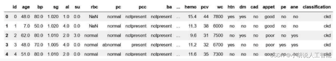
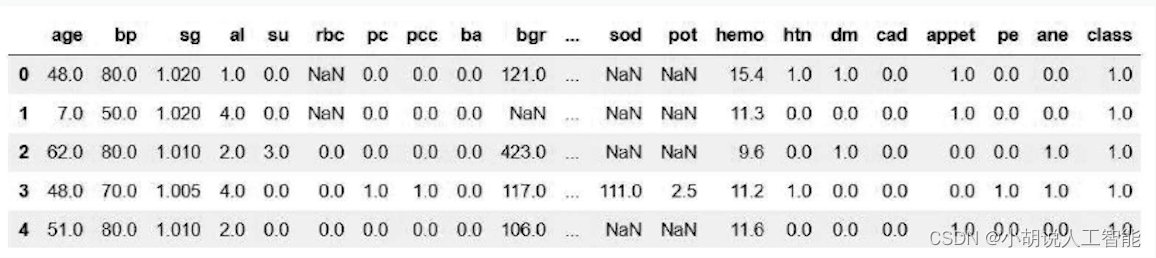
The chronic kidney disease data set is read through Pandas, and the successful reading effect is shown in the figure.

#读取肾病数据集
df = pd.read_csv("../Thursday9 10 11/kidney_disease.csv")
df.head()

The data types are processed, for example, the appetite (appet) data is good and poor, the pus cell cluster (pcc) is notpresent and present, and the categorical variables are converted into dummy variables 0 and 1.

#yes/no; abnormal/normal;present/notpresent;good/poor都转换为0/1
df[['htn','dm','cad','pe','ane']] = df[['htn','dm','cad','pe','ane']].replace(to_replace={
    
    'yes':1,'no':0})
df[['rbc','pc']] = df[['rbc','pc']].replace(to_replace={
    
    'abnormal':1,'normal':0})
df[['pcc','ba']] = df[['pcc','ba']].replace(to_replace={
    
    'present':1,'notpresent':0})
df[['appet']] = df[['appet']].replace(to_replace={
    
    'good':1,'poor':0,'no':np.nan})
df['classification'] = df['classification'].replace(to_replace={
    
    'ckd':1.0,'ckd\t':1.0,'notckd':0.0,'no':0.0})
df.rename(columns={
    
    'classification':'class'},inplace=True)
#将对患病有积极作用的变量设为0
df['pe'] = df['pe'].replace(to_replace='good',value=0)
df['appet'] = df['appet'].replace(to_replace='no',value=0)
df['cad'] = df['cad'].replace(to_replace='\tno',value=0)
df['dm'] = df['dm'].replace(to_replace={
    
    '\tno':0,'\tyes':1,' yes':1, '':np.nan})
#ID列去掉，为了表格中数据条理清晰而建立的变量
df.drop('id',axis=1,inplace=True)

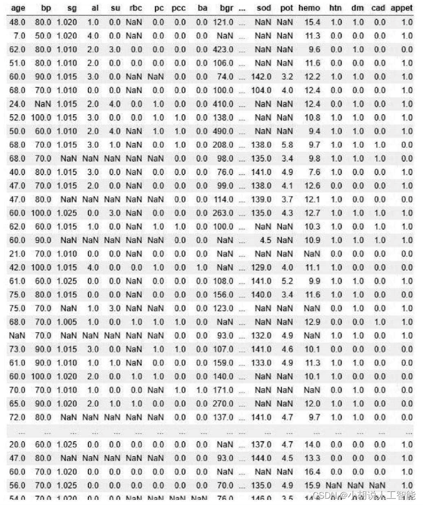
As shown in the figure after successful conversion.

Variables that check for default values ​​are shown in the image below. It can be seen from the figure that the number of default values ​​is not small. Since the data set is not large, the mean normalization method needs to be used to fill in the default values ​​by taking the average of all measured values ​​for patients and normal people.

#对病人所有测量值取均值
average0_age = df.loc[df['class'] ==True, 'age'].mean()
average0_bp = df.loc[df['class'] == True, 'bp'].mean()
average0_sg = df.loc[df['class'] == True, 'sg'].mean()
average0_al = df.loc[df['class'] == True, 'al'].mean()
average0_su = df.loc[df['class'] == True, 'su'].mean()
average0_rbc = df.loc[df['class'] == True, 'rbc'].mean()
average0_pc = df.loc[df['class'] == True, 'pc'].mean()
average0_pcc = df.loc[df['class'] == True, 'pcc'].mean()
average0_ba = df.loc[df['class'] == True, 'ba'].mean()
average0_bgr = df.loc[df['class'] == True, 'bgr'].mean()
average0_bu = df.loc[df['class'] == True, 'bu'].mean()
average0_sc = df.loc[df['class'] == True, 'sc'].mean()
average0_sod = df.loc[df['class'] == True, 'sod'].mean()
average0_pot = df.loc[df['class'] == True, 'pot'].mean()
average0_hemo = df.loc[df['class'] == True, 'hemo'].mean()
average0_htn = df.loc[df['class'] == True, 'htn'].mean()
average0_dm = df.loc[df['class'] == True, 'dm'].mean()
average0_cad = df.loc[df['class'] == True, 'cad'].mean()
average0_appet = df.loc[df['class'] ==True, 'appet'].mean()
average0_pe = df.loc[df['class'] == True, 'pe'].mean()
average0_ane = df.loc[df['class'] == True, 'ane'].mean()
#对正常人所有测量值取均值
average1_age = df.loc[df['class'] == False, 'age'].mean()
average1_bp = df.loc[df['class'] ==  False, 'bp'].mean()
average1_sg = df.loc[df['class'] ==  False, 'sg'].mean()
average1_al = df.loc[df['class'] ==  False, 'al'].mean()
average1_su = df.loc[df['class'] == False, 'su'].mean()
average1_rbc = df.loc[df['class'] == False, 'rbc'].mean()
average1_pc = df.loc[df['class'] ==  False, 'pc'].mean()
average1_pcc = df.loc[df['class'] ==  False, 'pcc'].mean()
average1_ba = df.loc[df['class'] ==  False, 'ba'].mean()
average1_bgr = df.loc[df['class'] ==  False, 'bgr'].mean()
average1_bu = df.loc[df['class'] ==  False, 'bu'].mean()
average1_sc = df.loc[df['class'] ==  False, 'sc'].mean()
average1_sod = df.loc[df['class'] ==  False, 'sod'].mean()
average1_pot = df.loc[df['class'] == False, 'pot'].mean()
average1_hemo = df.loc[df['class'] ==  False, 'hemo'].mean()
average1_htn = df.loc[df['class'] == False, 'htn'].mean()
average1_dm = df.loc[df['class'] ==  False, 'dm'].mean()
average1_cad = df.loc[df['class'] ==  False, 'cad'].mean()
average1_appet = df.loc[df['class'] ==  False, 'appet'].mean()
average1_pe = df.loc[df['class'] ==  False, 'pe'].mean()
average1_ane = df.loc[df['class'] ==  False, 'ane'].mean()
#根据是患者还是正常人，求出的均值赋给所有缺省值。如果为null，则取均值
df.loc[(df['class']==True)&(df['age'].isnull()),'age']= average0_age
df.loc[(df['class']==True)&(df['bp'].isnull()),'bp']= average0_bp
df.loc[(df['class']==True)&(df['sg'].isnull()),'sg']= average0_sg
df.loc[(df['class']==True)&(df['al'].isnull()),'al']= average0_al
df.loc[(df['class']==True)&(df['su'].isnull()),'su']= average0_su
df.loc[(df['class']==True)&(df['rbc'].isnull()),'rbc']= average0_rbc
df.loc[(df['class']==True)&(df['pc'].isnull()),'pc']= average0_pc
df.loc[(df['class']==True)&(df['pcc'].isnull()),'pcc']= average0_pcc
df.loc[(df['class']==True)&(df['ba'].isnull()),'ba']= average0_ba
df.loc[(df['class']==True)&(df['bgr'].isnull()),'bgr']= average0_bgr
df.loc[(df['class']==True)&(df['bu'].isnull()),'bu']= average0_bu
df.loc[(df['class']==True) &(df['sc'].isnull()),'sc']= average0_sc
df.loc[(df['class']==True)&(df['sod'].isnull()),'sod']= average0_sod
df.loc[(df['class']==True)&(df['pot'].isnull()),'pot']= average0_pot
df.loc[(df['class']==True) &(df['hemo'].isnull()),'hemo'] =average0_hemo
df.loc[(df['class']==True) &(df['htn'].isnull()),'htn'] = average0_htn
df.loc[(df['class']==True) &(df['dm'].isnull()),'dm'] = average0_dm
df.loc[(df['class']==True) &(df['cad'].isnull()),'cad'] = average0_cad
df.loc[(df['class']==True)&(df['appet'].isnull()),'appet']=average0_appet
df.loc[(df['class']==True)&(df['pe'].isnull()),'pe'] = average0_pe
df.loc[(df['class']==True) &(df['ane'].isnull()),'ane'] = average0_ane
#正常人
df.loc[(df['class']==False)&(df['age'].isnull()),'age']= average1_age
df.loc[(df['class'] ==False)  &(df['bp'].isnull()),'bp'] = average1_bp
df.loc[(df['class'] ==False)  &(df['sg'].isnull()),'sg'] = average1_sg
df.loc[(df['class'] ==False) &(df['al'].isnull()),'al'] = average1_al
df.loc[(df['class'] ==False)  &(df['su'].isnull()),'su'] = average1_su
df.loc[(df['class'] ==False) &(df['rbc'].isnull()),'rbc'] = average1_rbc
df.loc[(df['class'] ==False) &(df['pc'].isnull()),'pc'] = average1_pc
df.loc[(df['class'] ==False)&(df['pcc'].isnull()),'pcc'] = average1_pcc
df.loc[(df['class'] ==False)&(df['ba'].isnull()),'ba'] = average1_ba
df.loc[(df['class'] ==False&(df['bgr'].isnull()),'bgr'] = average1_bgr
df.loc[(df['class'] ==False)&(df['bu'].isnull()),'bu'] = average1_bu
df.loc[(df['class'] ==False)&(df['sc'].isnull()),'sc'] = average1_sc
df.loc[(df['class'] ==False)&(df['sod'].isnull()),'sod'] = average1_sod
df.loc[(df['class'] ==False)&(df['pot'].isnull()),'pot'] = average1_pot
df.loc[(df['class'] ==False)&(df['hemo'].isnull()),'hemo']= average1_hemo
df.loc[(df['class'] ==False)&(df['htn'].isnull()),'htn'] = average1_htn
df.loc[(df['class'] ==False)&(df['dm'].isnull()),'dm'] = average1_dm
df.loc[(df['class'] ==False) &(df['cad'].isnull()),'cad'] = average1_cad
df.loc[(df['class']==False)&(df['appet'].isnull()),'appet']=average1_appet
df.loc[(df['class'] ==False) &(df['pe'].isnull()),'pe'] = average1_pe
df.loc[(df['class'] ==False)  &(df['ane'].isnull()),'ane'] = average1_ane
#再次检查是否有缺省值
df.loc[(df['age'].isnull()) |
        (df['bp'].isnull()) |
        (df['sg'].isnull()) |
        (df['al'].isnull()) |
        (df['su'].isnull()) |
        (df['rbc'].isnull()) |
        (df['pc'].isnull()) |
        (df['pcc'].isnull()) |
        (df['ba'].isnull()) |
        (df['bgr'].isnull()) |
        (df['bu'].isnull()) |
        (df['sc'].isnull()) |
        (df['sod'].isnull()) |
        (df['pot'].isnull()) |
        (df['hemo'].isnull()) |
        (df['htn'].isnull()) |
        (df['dm'].isnull()) |
        (df['cad'].isnull()) |
        (df['appet'].isnull()) |
        (df['pe'].isnull()) |
        (df['ane'].isnull()) |
        (df['class'].isnull())]
#使用Scikit-learn的train_test_split()函数自动划分训练集和测试集
X_train, X_test, y_train, y_test = train_test_split(df.iloc[:,:-1], df['class'],test_size = 0.33, random_state=44,stratify= df['class'] )
#慢性肾病数据预处理完成

2) Model training and saving

After loading the data into the model, you need to define the model structure, find optimization parameters and save the model.

Define model structure

This section includes the Heart Disease Data Set Definition Model and the Chronic Kidney Disease Data Set Definition Model.

Heart Disease Dataset Definition Model

The relevant code is as follows:

#由于一次尝试过多参数会导致内存不足，所以分段寻找最大值
num=np.zeros(20,int)
for i in range(0,20):
    num[i]=i
"""
每次将num扩大20，迭代改变随机森林中树的数量以及权重分配等参数。使用GridSearchCV自动寻找最优参数。
"""
from sklearn.ensemble import RandomForestClassifier
from sklearn.model_selection import train_test_split, GridSearchCV
tuned_parameters = [{
    
    'n_estimators':num,'class_weight':[None,{
    
    0: 0.33,1:0.67},'balanced'],'random_state':[1]}]
rf = GridSearchCV(RandomForestClassifier(), tuned_parameters, cv=10,scoring='f1')
rf.fit(x_train.T, y_train.T)
print('Best parameters:')
print(rf.best_params_)
#训练完成后，使用print()函数输出最佳参数，森林中有1005棵树的时候准确率最高
#保存最优参数，将最佳参数带入模型进行训练
rf_best = rf.best_estimator_
rf_best.fit(x_train.T, y_train.T)
acc = rf.score(x_test.T,y_test.T)*100
accuracies['Random Forest'] = acc
print("Random Forest Algorithm Accuracy Score : {:.2f}%".format(acc))
#最佳参数的模型训练完成后，在测试集上计算模型准确率，达89.86%

Chronic kidney disease dataset definition model

The relevant code is as follows:

#寻找随机森林最优参数
tuned_parameters= [{
    
    'n_estimators':[7,8,9,10,11,12,13,14,15,16],'max_depth':[2,3,4,5,6,None],'class_weight':[None,{
    
    0: 0.33,1:0.67},'balanced'],'random_state':[42]}]
clf = GridSearchCV(RandomForestClassifier(), tuned_parameters, cv=10,scoring='f1')
clf.fit(X_train, y_train)
print('Best parameters:')
print(clf.best_params_)
#训练完成后，使用print()函数输出最佳参数，随机森林中有7棵树时准确率最高
#将最优参数带入模型进行训练
accuracies = {
    
    }
rf = RandomForestClassifier(class_weight=None, max_depth= 6,n_estimators = 7, random_state = 42)
rf.fit(X_train, y_train)
acc = rf.score(X_test, y_test)*100
accuracies['Random Forest'] = acc
print("Random Forest Algorithm Accuracy Score : {:.2f}%".format(acc))
#最佳参数的模型训练完成后，在测试集上计算模型准确率，达100%

Save model

In order to be read by the Python program, the model needs to be saved as a .pkl format file, and the module in the pickle library is used to save the model.

Heart disease model saving

The relevant code is as follows:

import pickle
with open("model.pkl", "wb") as f:
    pickle.dump(rf, f)

Chronic kidney disease dataset definition model

The relevant code is as follows:

import pickle
with open("model_kidney.pkl", "wb") as f:
    pickle.dump(rf, f)

3) Model application

For human diseases, the risk of misdiagnosis is huge. If the accuracy rate is not 100%, it will be a loss for the patient. However, in the past, just predicting whether to suffer from a disease was a two-classification problem. In principle, machine predictions of diseases are based on the weight of various indicators. This project makes full use of the advantages of machine learning, multiplying and summing the importance of each feature and the value of each indicator to obtain a weighted value. Within the program, the average value of each indicator and the importance of the corresponding features of patients and normal people are weighted and summed in advance to obtain the average level of patients and normal people. After the user is qualitatively judged to be a patient, the user's numerical values ​​are compared with the patient average, and the severity of the user's condition relative to most patients is quantitatively given; if the user is judged to be a normal person, his various numerical values ​​are compared with the normal average. Make a comparison and give the user's sub-health level compared to most normal people. After processing, it not only achieves qualitative judgment, but also quantifies the user situation. On the one hand, it prevents risks caused by accidental misdiagnosis; on the other hand, it gives patients hope to fight the disease and sounds a warning to people with normal physical examinations about sub-health.

Innovation in application of chronic kidney disease models

#通过eli5得到各特征重要性
import eli5 
from eli5.sklearn import PermutationImportance
perm = PermutationImportance(rf, random_state=1).fit(x_test.T, y_test.T)
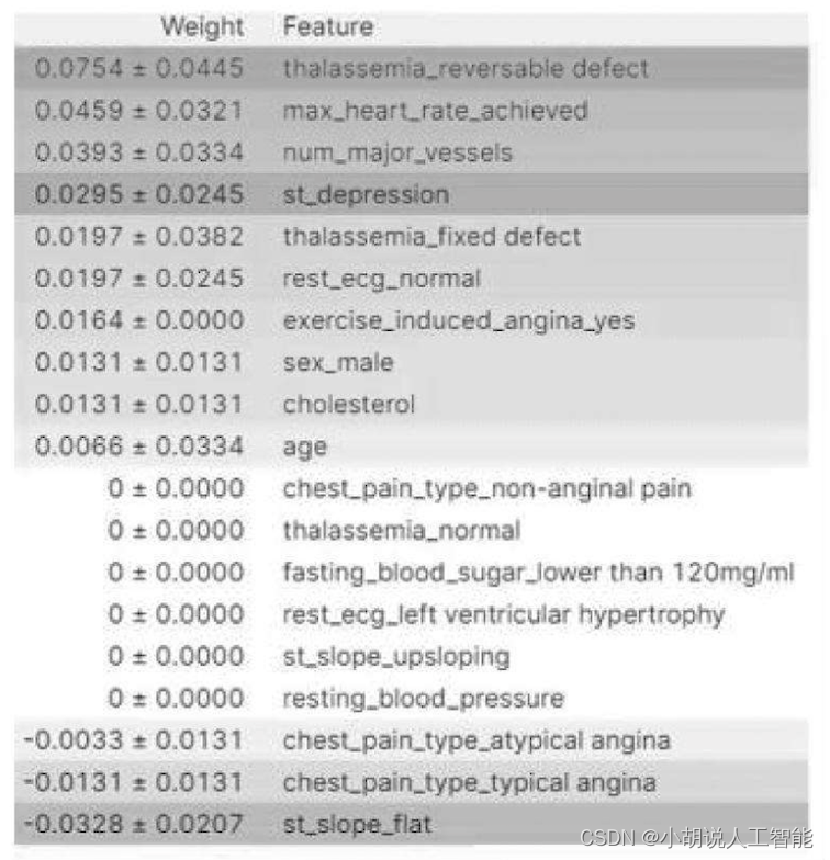
eli5.show_weights(perm, feature_names = x_test.T.columns.tolist())

The importance of each feature output is shown in Figure 3. It can be seen from the figure that the age factor has no impact on the disease, which is consistent with common sense. Then the average values ​​of patients and normal subjects were obtained respectively, as shown in Figure 4.

Figure 3 Importance of heart disease characteristics

Figure 4 Average values ​​of heart disease patients and normal people

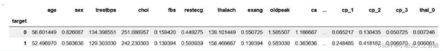
#求均值
df.groupby('target').mean()
#正常人平均水平
average0_count=np.multiply(average0,w)
average0_sum=sum(average0_count)
#病人平均水平
average1_count=np.multiply(average1,w)
average1_sum=sum(average1_count)
#输出得到的数值
print(average1_sum) #患者
print(average0_sum) #正常人

The weighted summation values ​​of patients and normal subjects are shown in the figure.

Save this value, and when the user uses it, after judging whether it is a patient or a normal person, the specific situation will be quantitatively determined based on the ratio.

Innovation in application of chronic kidney disease models

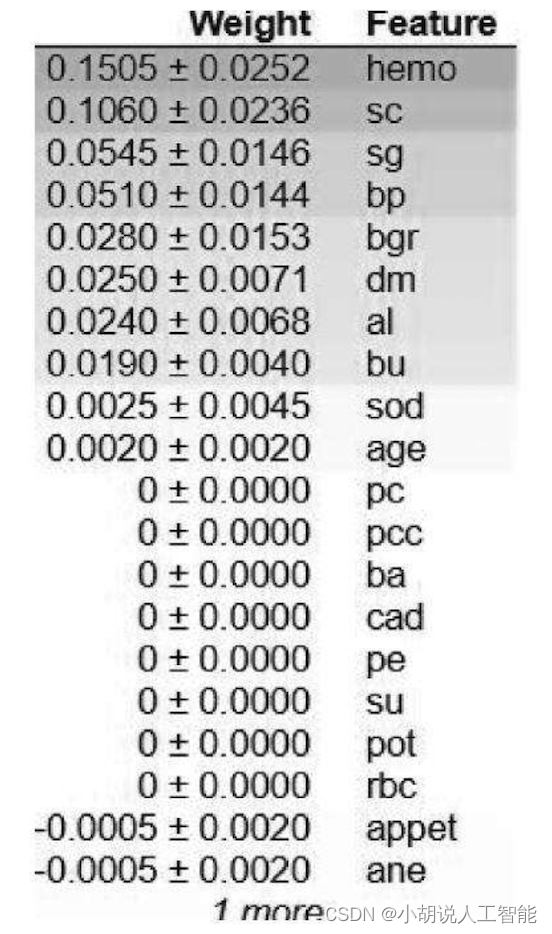
The importance of each feature is obtained through eli5, and the output importance of each feature is shown in the figure.

import eli5 
from eli5.sklearn import PermutationImportance
perm = PermutationImportance(rf, random_state=1).fit(x_test.T, y_test.T)
eli5.show_weights(perm, feature_names = x_test.T.columns.tolist())
import eli5 #for purmutation importance
from eli5.sklearn import PermutationImportance
perm = PermutationImportance(rf, random_state=1).fit(X_test, y_test)
eli5.show_weights(perm, feature_names = X_test.columns.tolist())

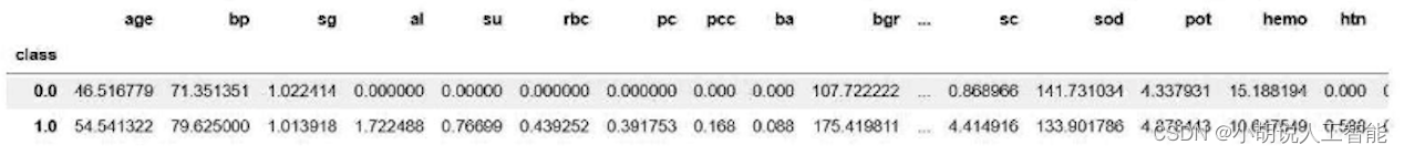
The average values ​​of patients and normal subjects were obtained respectively, as shown in the figure.

#求均值
#正常人平均水平
average0_count=np.multiply(average0,w)
average0_sum=sum(average0_count)
#病人平均水平
average1_count=np.multiply(average1,w)
average1_sum=sum(average1_count)
print(average1_sum)#患者
print(average0_sum)#正常人
#输出得到的数值
print(average1_sum)#病人
print(average0_sum)#正常人

The weighted summation values ​​of patients and normal subjects are shown in the figure.

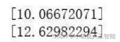
Save this value. When the user uses it, after judging whether it is a patient or a normal person, the specific situation can be quantified based on the ratio.

Other related blogs

• Based on random forest + small intelligent health recommendation assistant (heart disease + chronic kidney disease health prediction + drug recommendation) - machine learning algorithm application (including Python engineering source code) + data set (2)

• Based on random forest + small intelligent health recommendation assistant (heart disease + chronic kidney disease health prediction + drug recommendation) - machine learning algorithm application (including Python engineering source code) + data set (3)

Project source code download

For details, please see my blog resource download page

---

Download other information

If you want to continue to understand the learning routes and knowledge systems related to artificial intelligence, you are welcome to read my other blog " Heavyweight | Complete Artificial Intelligence AI Learning - Basic Knowledge Learning Route, all information can be downloaded directly from the network disk without following any routines.》
This blog refers to Github’s well-known open source platform, AI technology platform and experts in related fields: Datawhale, ApacheCN, AI Youdao and Dr. Huang Haiguang, etc., which has nearly 100G of related information. I hope it can help all my friends.