The subtractive average optimizer of the optimization algorithm in 2023, the matlab code is directly copied, and compared with the gray wolf, particle swarm algorithm...

"  Today's protagonist is: the newly released optimization algorithm in April 2023 , " Subtractive Average Optimizer ", which is currently not found on HowNet. The algorithm is simple in principle and is very suitable for novices . Counting the initialization particles, there are only 4 formulas in total .But! Here comes the important point . Although the principle of this algorithm is simple, the optimization effect is excellent . The following will compare this algorithm with the particle swarm algorithm and gray wolf algorithm. "

01

—

Principle of Subtractive Average Optimizer

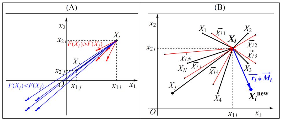
    The basic inspiration for the design of the Subtraction-Average-Based Optimizer (SABO) comes from mathematical concepts such as the mean, the difference in search agent positions, and the sign of the difference of two values ​​of the objective function.

• (1) Algorithm initialization

The particle initialization formula is the same as most intelligent optimization algorithms such as particle swarm optimization, which uses the rand function to randomly generate a bunch of particles within the range of the upper and lower limits.

• (2) SABO mathematical model

The SABO algorithm introduces a new calculation concept, "-v", which is called the v-subtraction between search agent B and search agent a, defined as follows:

is a vector with dimension m, which is a random number generated by [1, 2], F(A) and F(B) are the values ​​of the objective functions of search agents A and B respectively, and sign is the signum function.

In the SABO algorithm, the displacement of any search agent Xi in the search space is calculated by the arithmetic mean of the “-v” subtraction of each search agent Xj. The location update method is as follows:

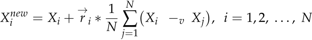
N is the total number of particles, and ri is a random value that obeys a normal distribution.

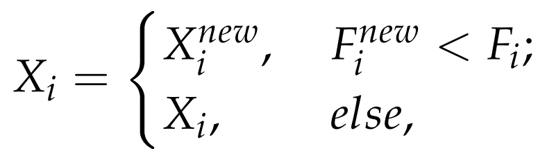
Particle position replacement formula, which is also consistent with most algorithms.

The mathematical model of the SABO algorithm is as follows:

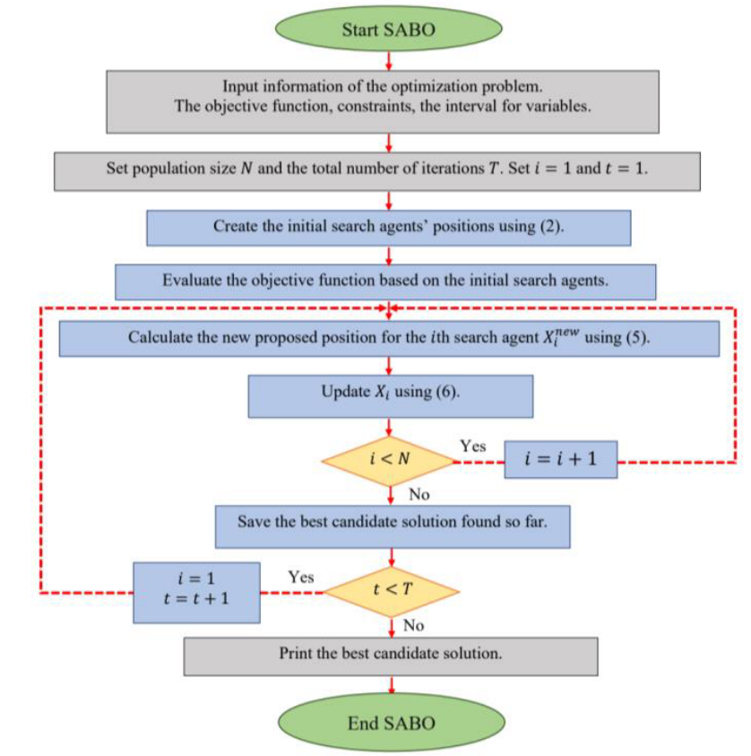
The flow chart of SABO algorithm is as follows:

02

—

SABO's optimization effect display

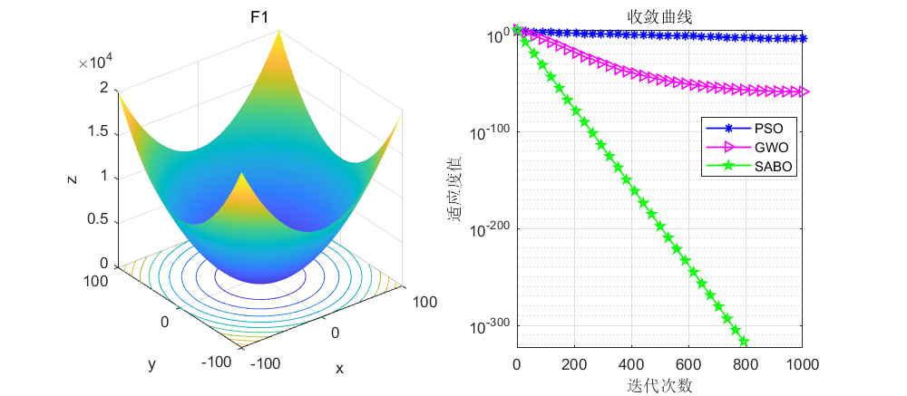
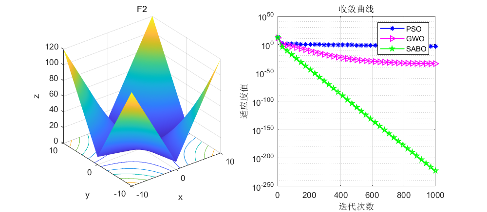
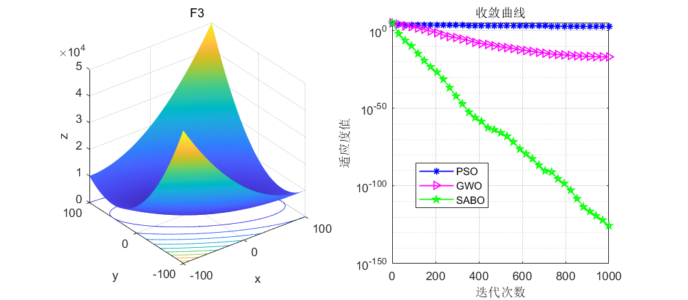
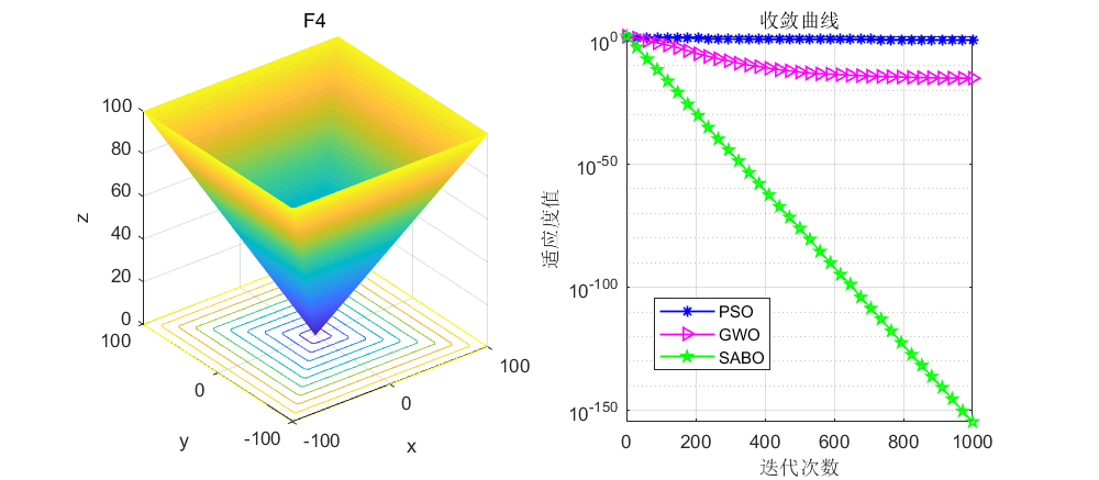
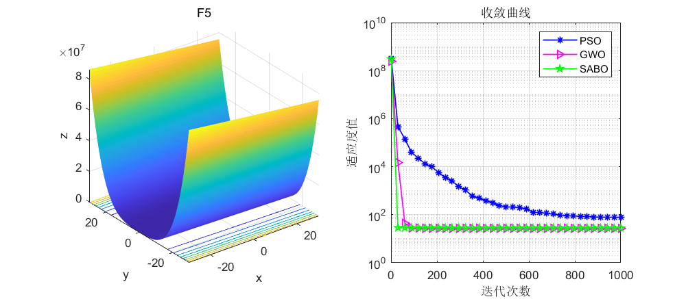
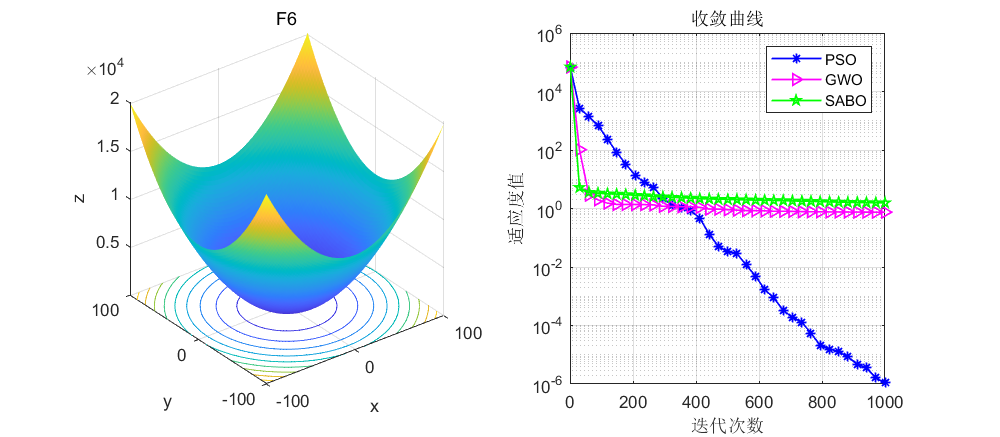
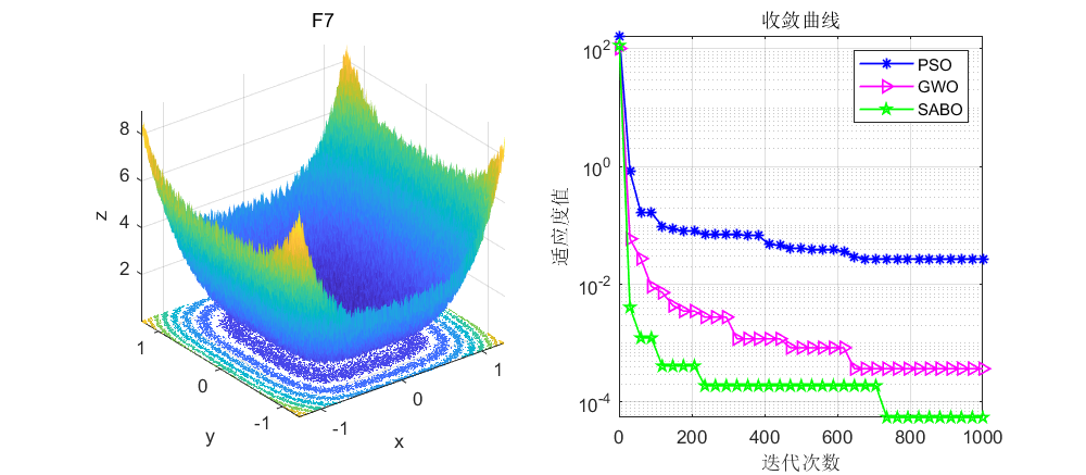
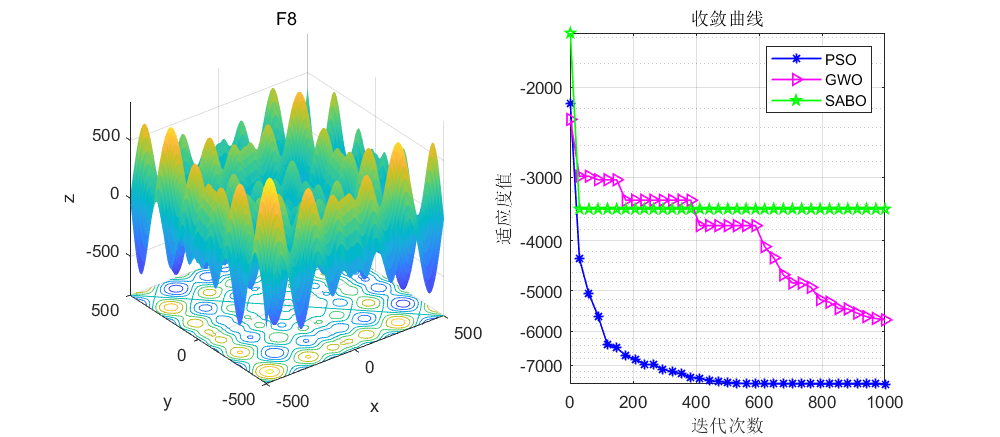
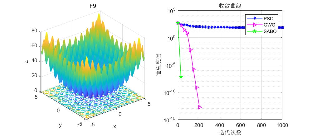
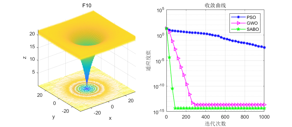
The test is still carried out on the CEC2005 function, the number of iterations of the algorithm is set to 1000, and the number of populations is 30.

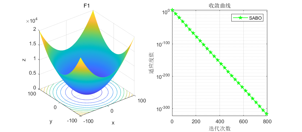
It can be seen from this F1 function that the SABO algorithm reaches 0 in about 800 times. Other algorithms are at most e-hundreds of powers, and rarely reach 0 directly. In addition, due to the simple principle of the SABO algorithm, its operation speed is extremely fast, you can try it yourself.

Next, directly compare the SABO algorithm with the gray wolf algorithm and the particle swarm algorithm. You can experience the quality of the SABO algorithm by yourself.

03

—

MATLAB code for SABO

function[Best_score,Best_pos,SABO_curve]=SABO(N,T,lo,hi,m,fitness)
lo=ones(1,m).*(lo);                              % Lower limit for variables
hi=ones(1,m).*(hi);                              % Upper limit for variables
%% INITIALIZATION
for i=1:m
    X(:,i) = lo(i)+rand(N,1).*(hi(i) - lo(i));                          % Initial population
end
for i =1:N
    L=X(i,:);
    fit(i)=fitness(L);
end
%%
for t=1:T  % algorithm iteration
   %%  update: BEST proposed solution
    [Fbest , blocation]=min(fit);
    if t==1
        xbest=X(blocation,:);                                           % Optimal location
        fbest=Fbest;                                           % The optimization objective function
    elseif Fbest<fbest
        fbest=Fbest;
        xbest=X(blocation,:);
    end
    %%
    DX=zeros(N,m);  
    for i=1:N
        %% based om Eq(4)
        for j=1:N
            I=round(1+rand+rand);
            for d=1:m
                DX(i,d)=DX(i,d)+(X(j,d)-I.*X(i,d)).*sign(fit(i)-fit(j));
            end
        end
        X_new_P1= X(i,:)+((rand(1,m).*DX(i,:))./(N));
        X_new_P1 = max(X_new_P1,lo);
        X_new_P1 = min(X_new_P1,hi);
        
        %% update position based on Eq (5)
        L=X_new_P1;
        fit_new_P1=fitness(L);
        if fit_new_P1<fit(i)
            X(i,:) = X_new_P1;
            fit(i) = fit_new_P1;
        end
        %%            
    end% end for i=1:N
    %%
    best_so_far(t)=fbest;
    average(t) = mean (fit);
    
end
Best_score=fbest;
Best_pos=xbest;
SABO_curve=best_so_far;
end

Here is still the core code directly, you can just copy it directly.

The literature of SABO algorithm, the MATLAB code of SABO, the comparison code of SABO algorithm, gray wolf algorithm and particle swarm algorithm are all packaged, and you can directly reply to the keywords to get it for free.

Click the card below to reply to the keyword to get the code, keyword: 2023

If you think the article is good, please leave a like for the author! Thanks!