Modificación del código de costura panorámica de imágenes múltiples

prefacio

Código de referencia: dirección del código github

1. Crea un entorno virtual

conda create -n stitching python=3.7.0

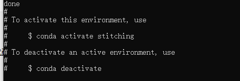
2. Activar el entorno virtual

conda activate stitching

3. Instalar opencv y los paquetes correspondientes

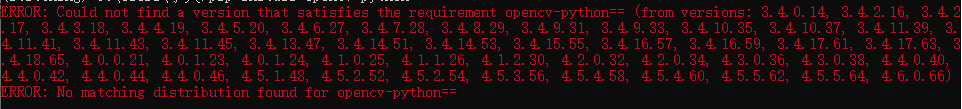
3.1 Ver la versión instalable de opencv

La última versión de la instalación de opencv correspondiente se puede ver instalación de opencv

pip install opencv-python==

instalar

pip install opencv-python==3.4.2.16

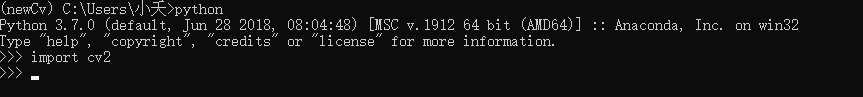
realizar pruebas

3.2 Instalar el paquete correspondiente

pip install imutils

3.3 Instalar opencv-contrib-python

La solución al error

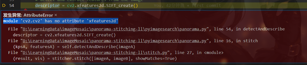
: agregue una versión del paquete contrib correspondiente

pip install opencv-contrib-python==3.4.2.16

3.4 instalación de matplotlib

pip install matplotlib

3.5 Instalación de PCV

Puede consultar la instalación de PCV

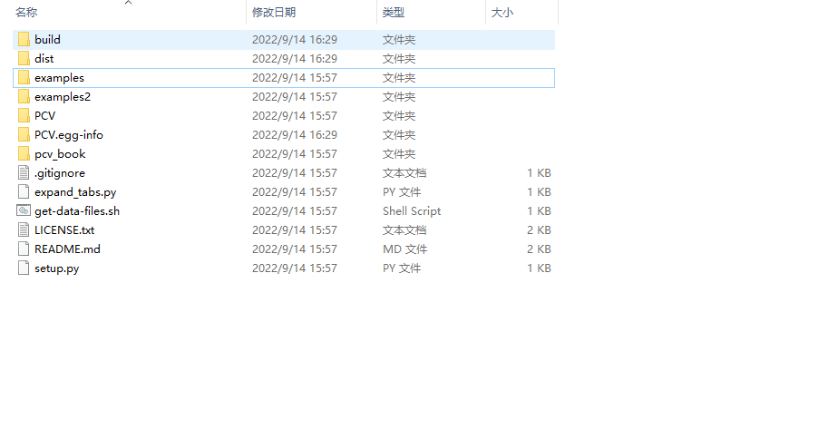
1. Ingrese el código PCV del clon de la carpeta correspondiente

git clone https://github.com/Li-Shu14/PCV.git

2. Instale
   aquí porque lo instalé en el entorno de Windows
   Primero cambie la letra de la unidad a su unidad correspondiente, como D:
   Ingrese a la carpeta cd xxx/PCV
   

python setup.py install

3.5 instalación espía

Volviendo al código de referencia, ocurrió un error al ejecutar el programa

ModuleNotFoundError: No module named 'scipy'

Instalar en el entorno correspondiente

pip install scipy

4. Registro de errores

4.1 error de impresión

SyntaxError: Missing parentheses in call to 'print'. Did you mean print('warp - right')?

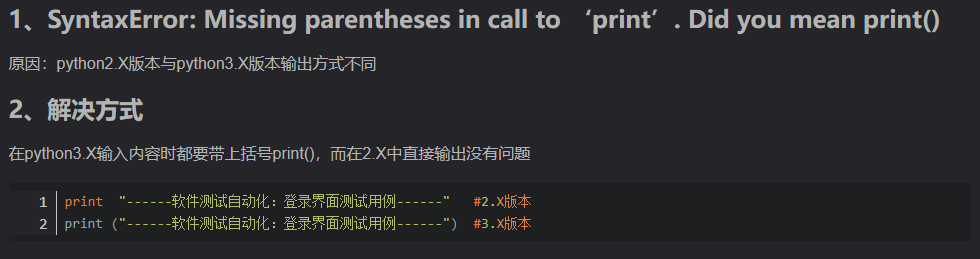
El PCV anterior se aplicó a python2, y ahora hay un PCV github basado en python3 actualizado para python3

Consulte la instalación de PCV para instalar en base a python3

4.2 matplotlib.delaunay informa de un error

ModuleNotFoundError: No module named 'matplotlib.delaunay'

Para el método de cambio, consulte matplotlib.delaunay para informar un error
y luego vuelva a instalar (no puede ingresar directamente el archivo correspondiente aquí, por lo que debe volver a instalar después de la modificación. Tengo un error en la instalación aquí. I eliminó directamente el entorno virtual y lo recreó, y luego lo instaló)

4.3 No se puede generar el archivo .sift

  File "D:\anaconda\envs\stitching\lib\site-packages\numpy\lib\_datasource.py", line 533, in open
    raise IOError("%s not found." % path)
OSError: ./test/1027-1.sift not found.

Enlace de referencia:
OSError: tamiz no encontrado resolución de problemas
enlace de referencia de unión de imágenes

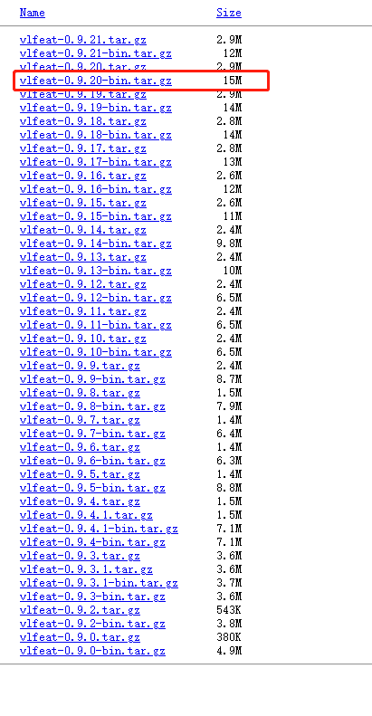
1. Descargar VLfeat Descargar
   VLfeat
   

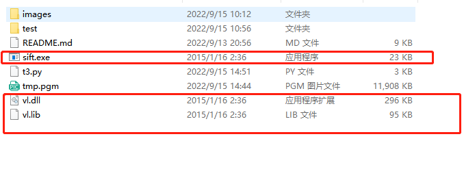
2. Seleccione el archivo correspondiente y muévalo a la carpeta del proyecto actual
   

3. 
   Busque la ruta de instalación directa del archivo [sift.py] en el directorio correspondiente según si su computadora está instalada directamente con Python o Anaconda : python\Lib\site-packages\PCV\localdescriptors
   Ruta de instalación de Anaconda :Anaconda\Lib\site-packages\PCV\localdescriptors

4. Abra sift.py, modifique la ruta
   Abra el archivo [sift.py], global cmmd , cambie la ruta entre comillas señaladas por la flecha a la ruta de [sift.exe] en su proyecto
   Nota: si usa "\" en la ruta, necesita Agregar "r" en la parte delantera, no se requiere usar ''/'' o "\" para
   
   
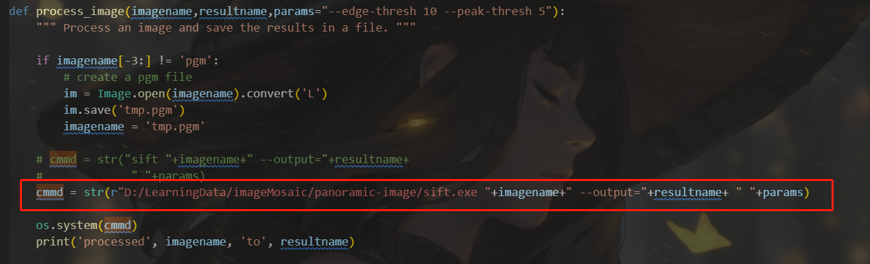
   generar correctamente el archivo de tamiz

cmmd = str(r"D:/LearningData/imageMosaic/panoramic-image/sift.exe "+imagename+" --output="+resultname+ " "+params) 

4.4 Las imágenes son demasiado diferentes

ValueError: did not meet fit acceptance criteria

La unión de múltiples imágenes tiene requisitos relativamente altos para las imágenes, y el efecto de la unión es deficiente si la diferencia es grande o demasiado pequeña (casi la misma). Y si la ubicación de disparo cambia demasiado, el valor de coincidencia será 0

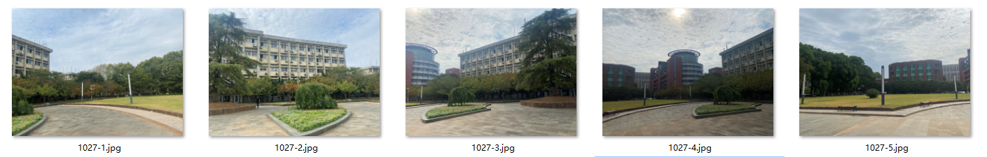
5. Resultado de empalme

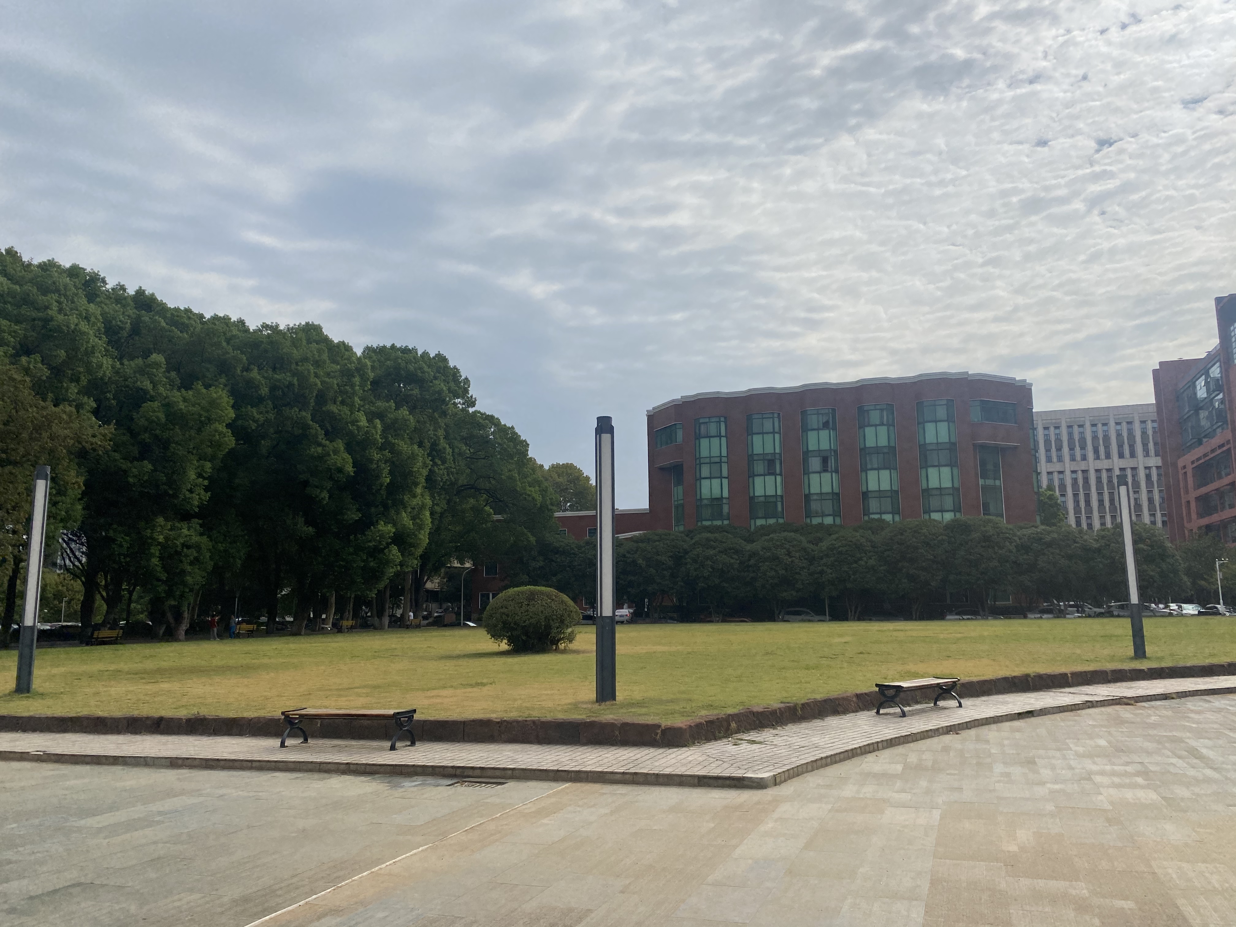
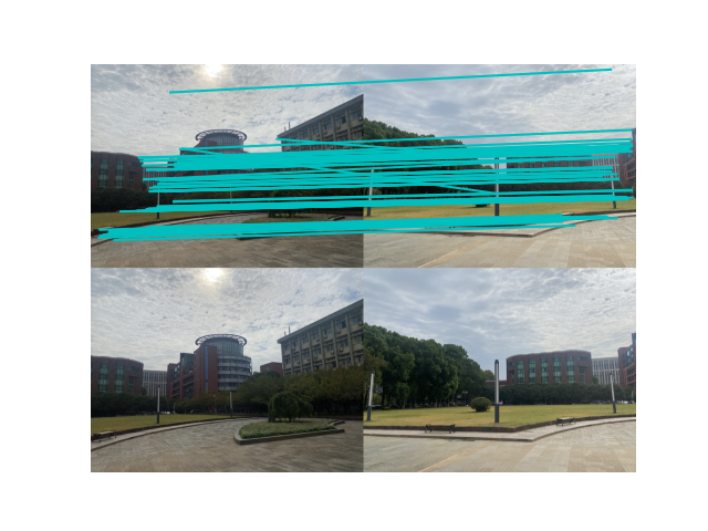
5.1 Unión de dos imágenes

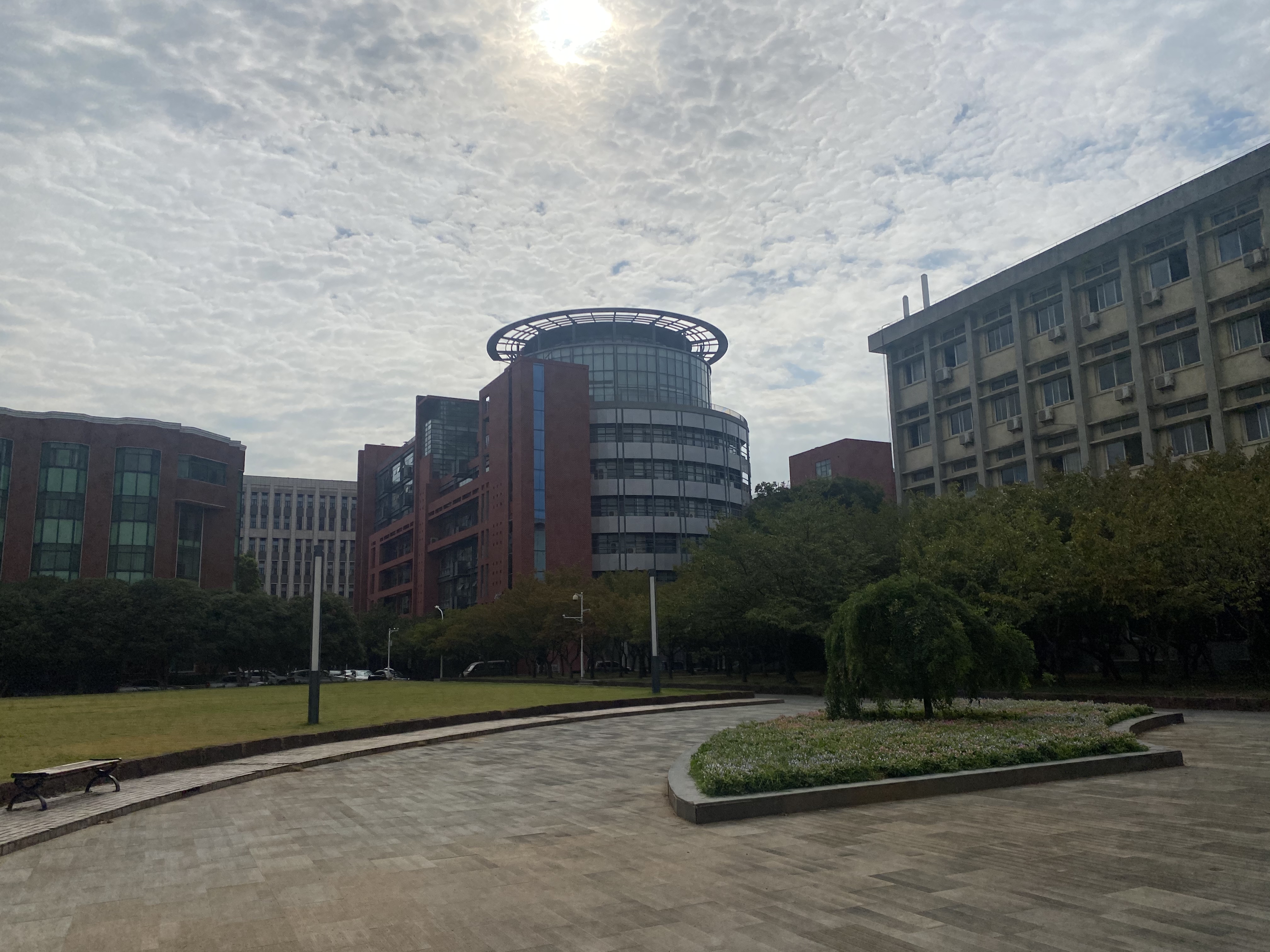
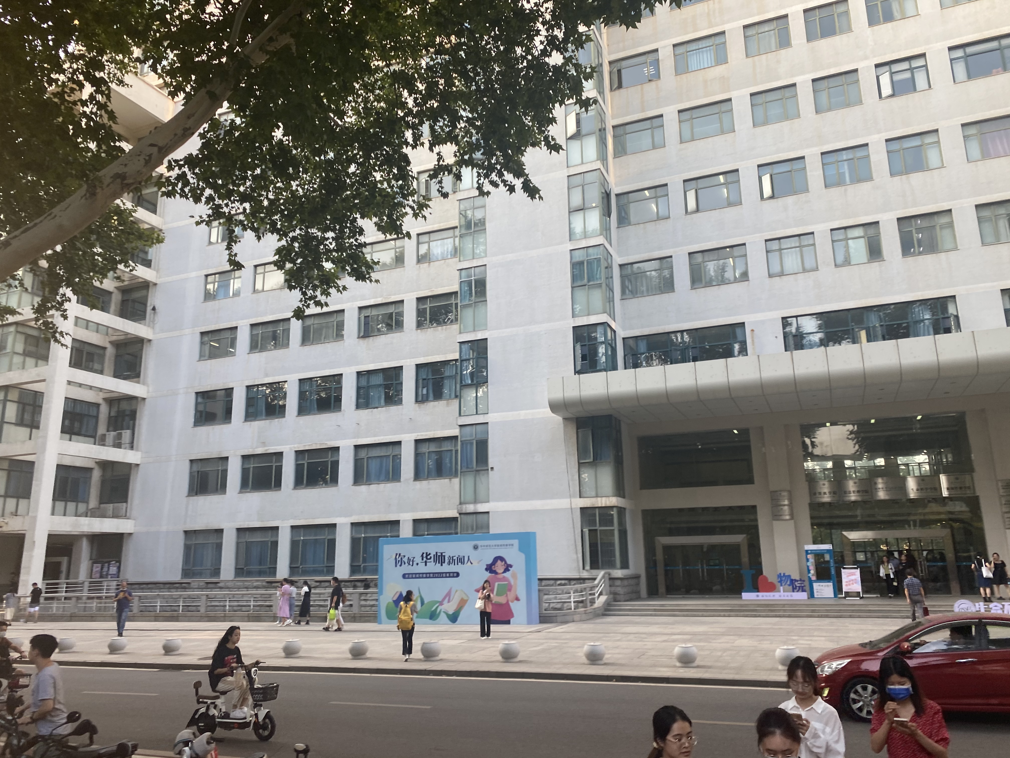
1. imagen original
   
   

2. obtener función
   

3. resultado de costura
   

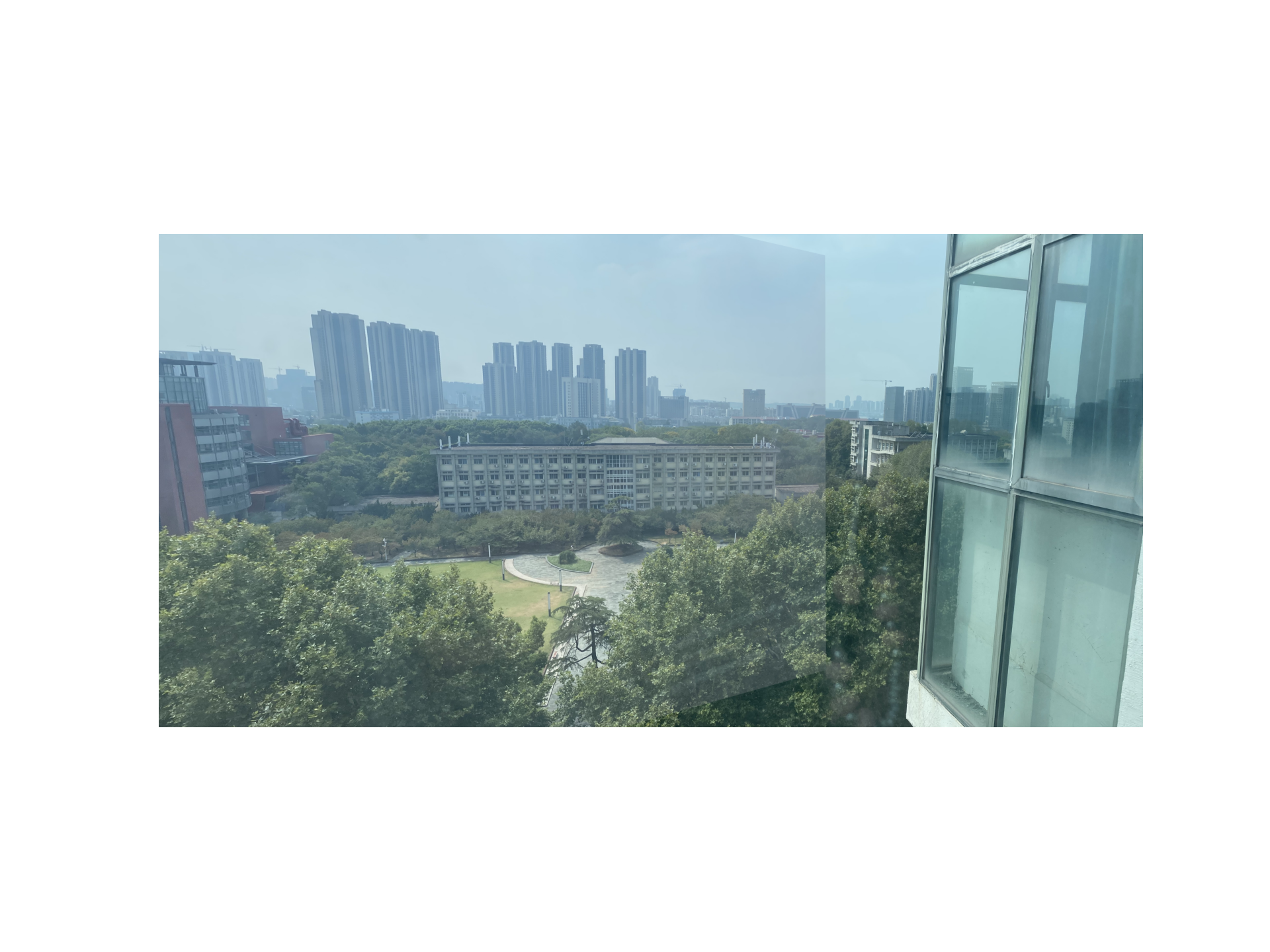
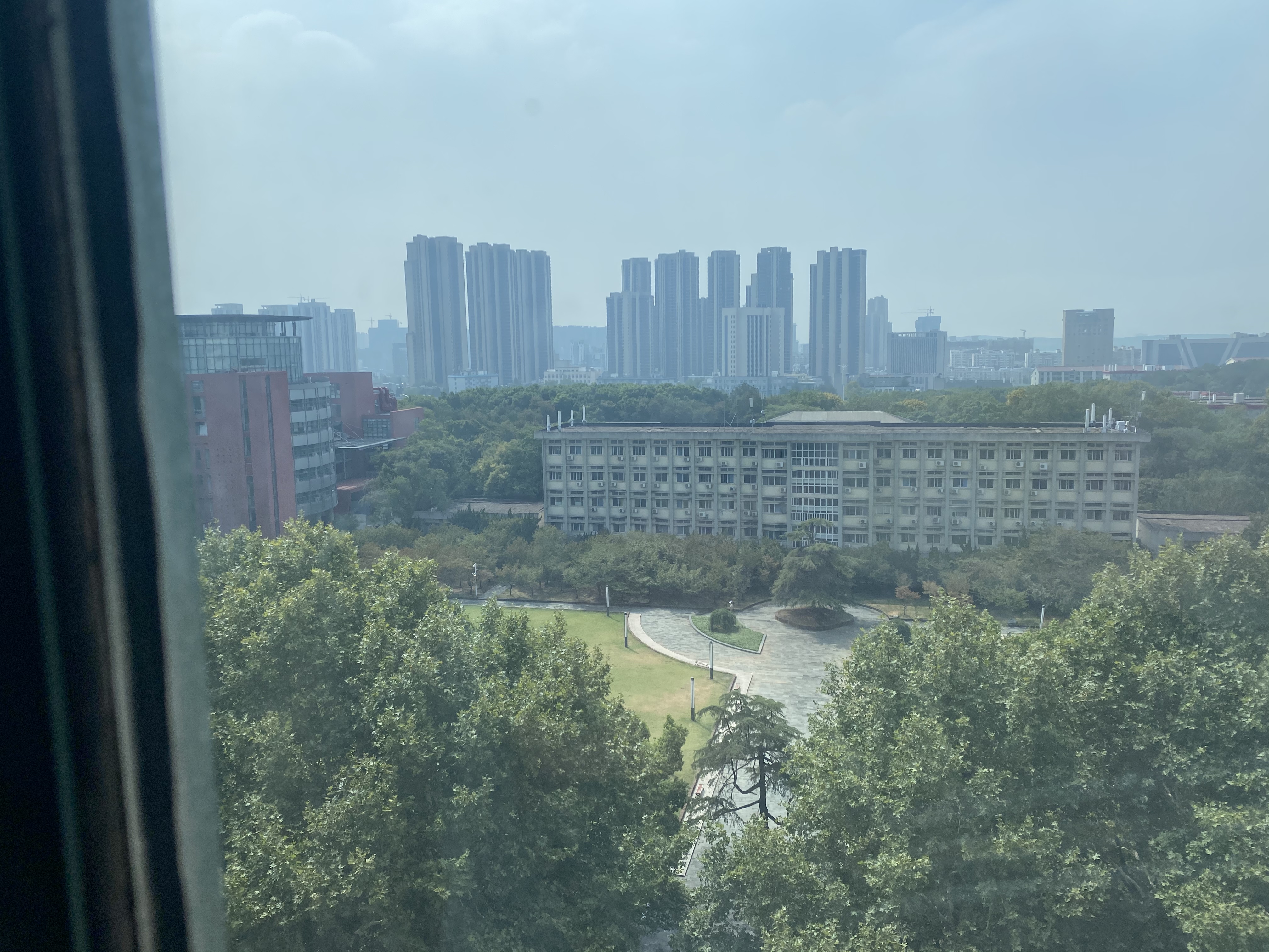
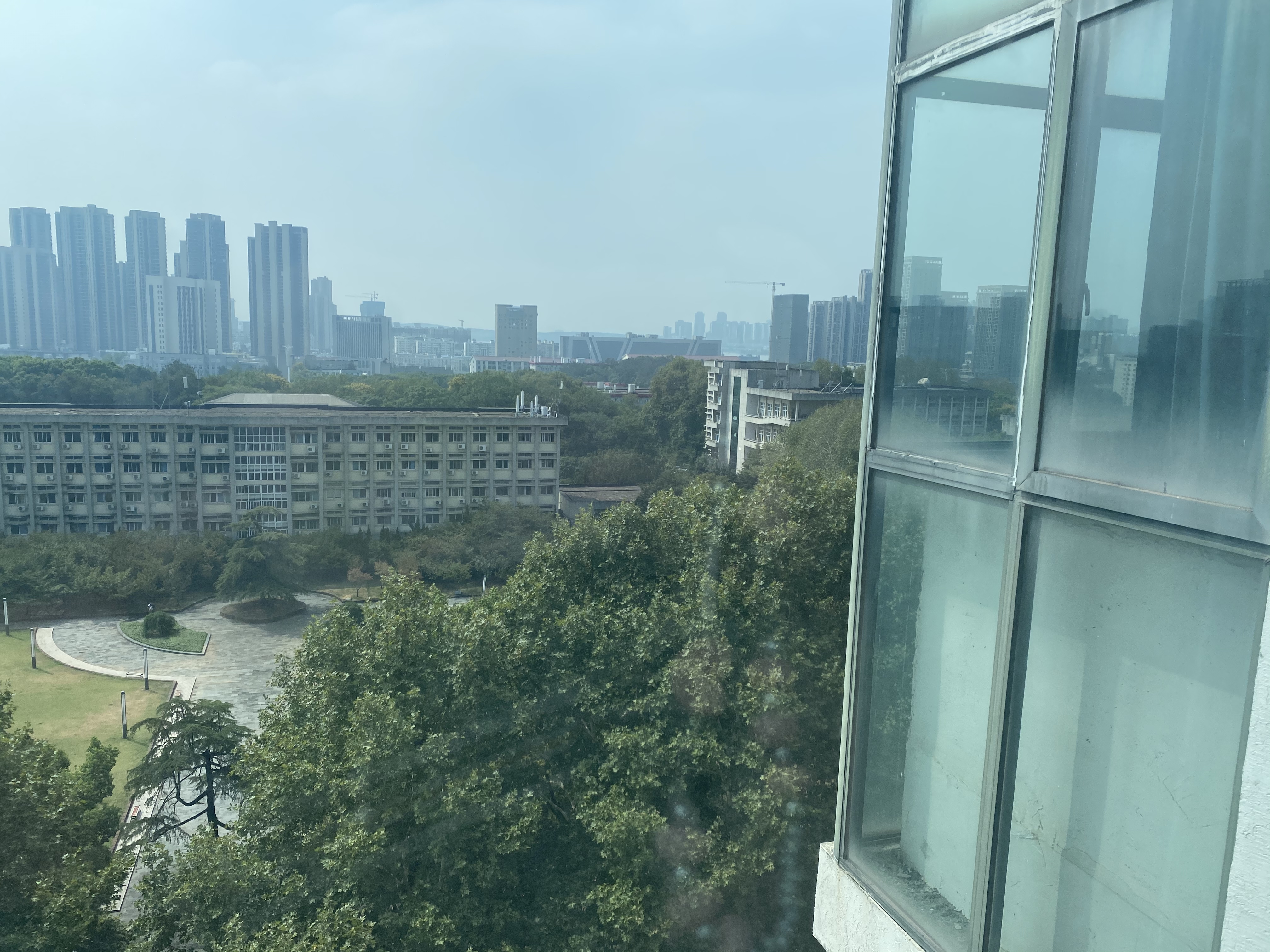
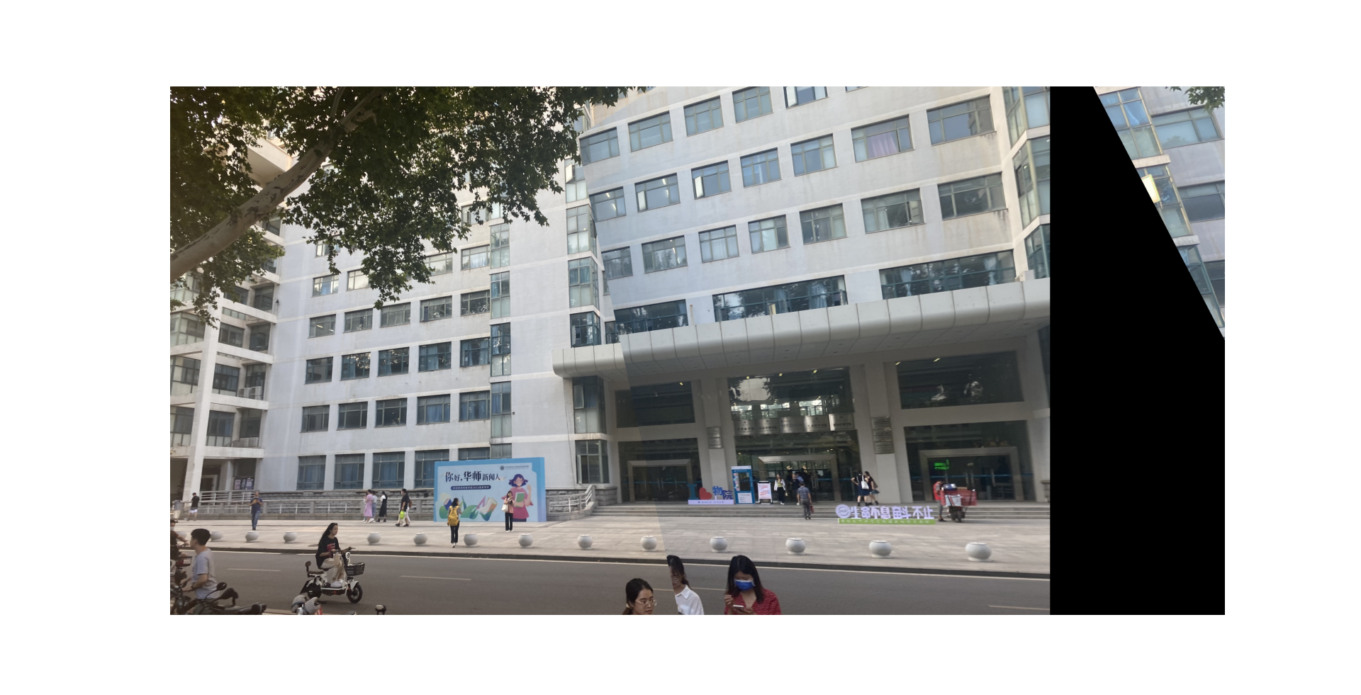
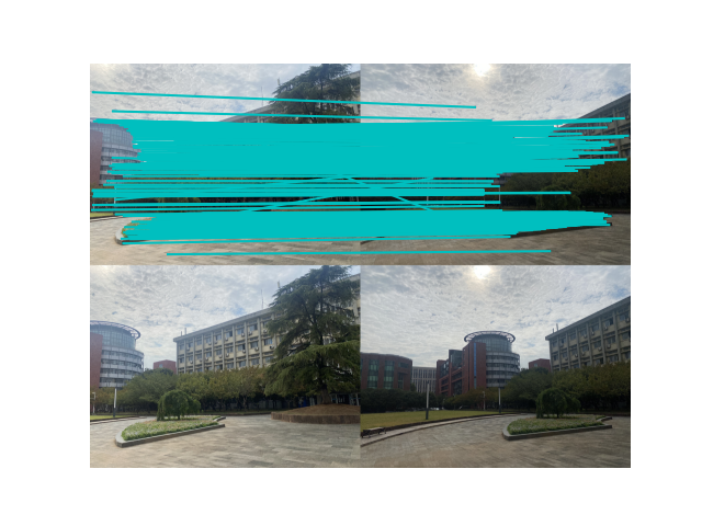
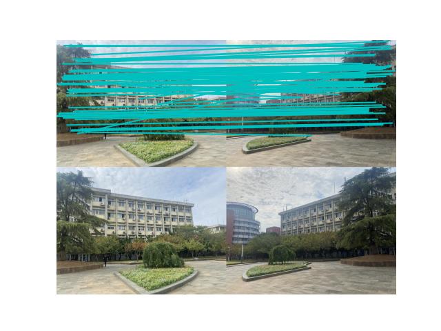
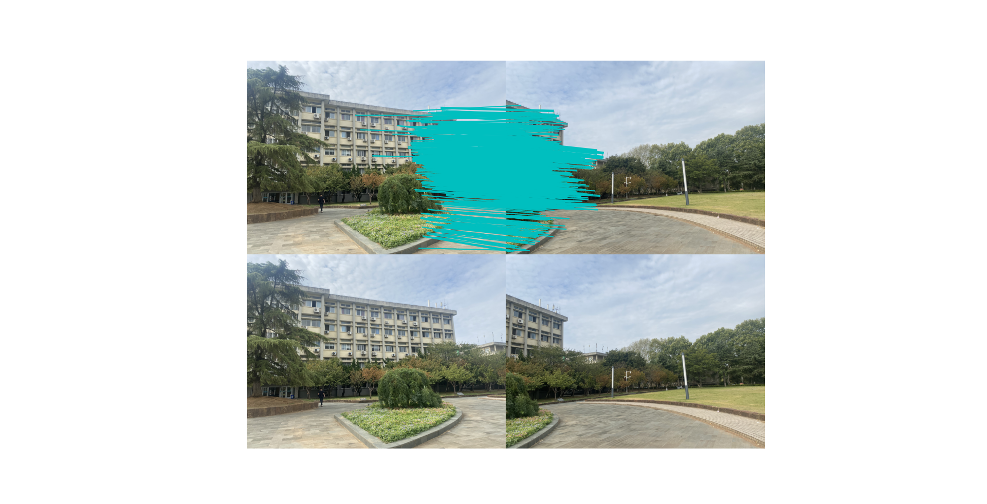
5.2 Unión de dos imágenes desde diferentes ángulos

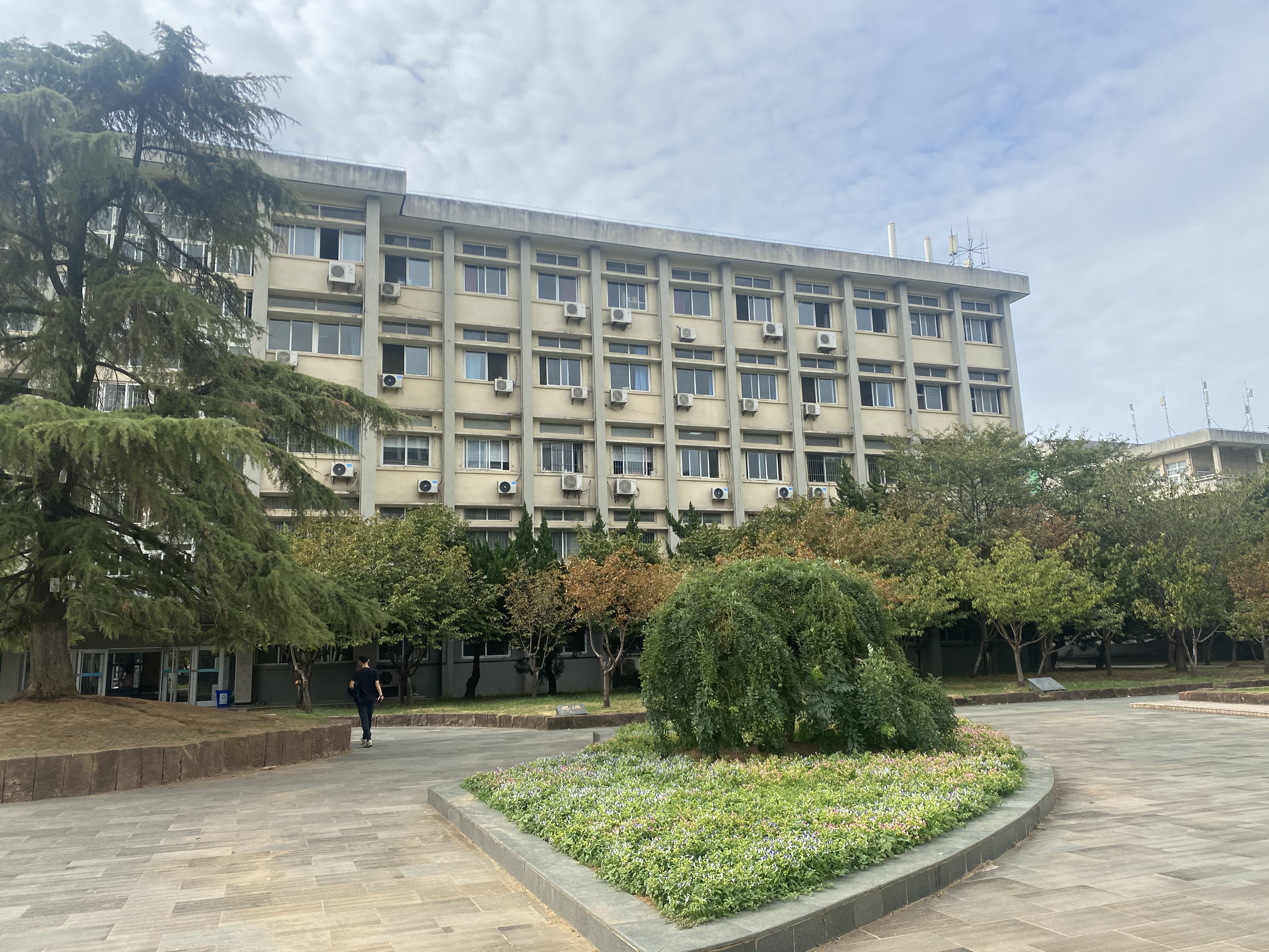
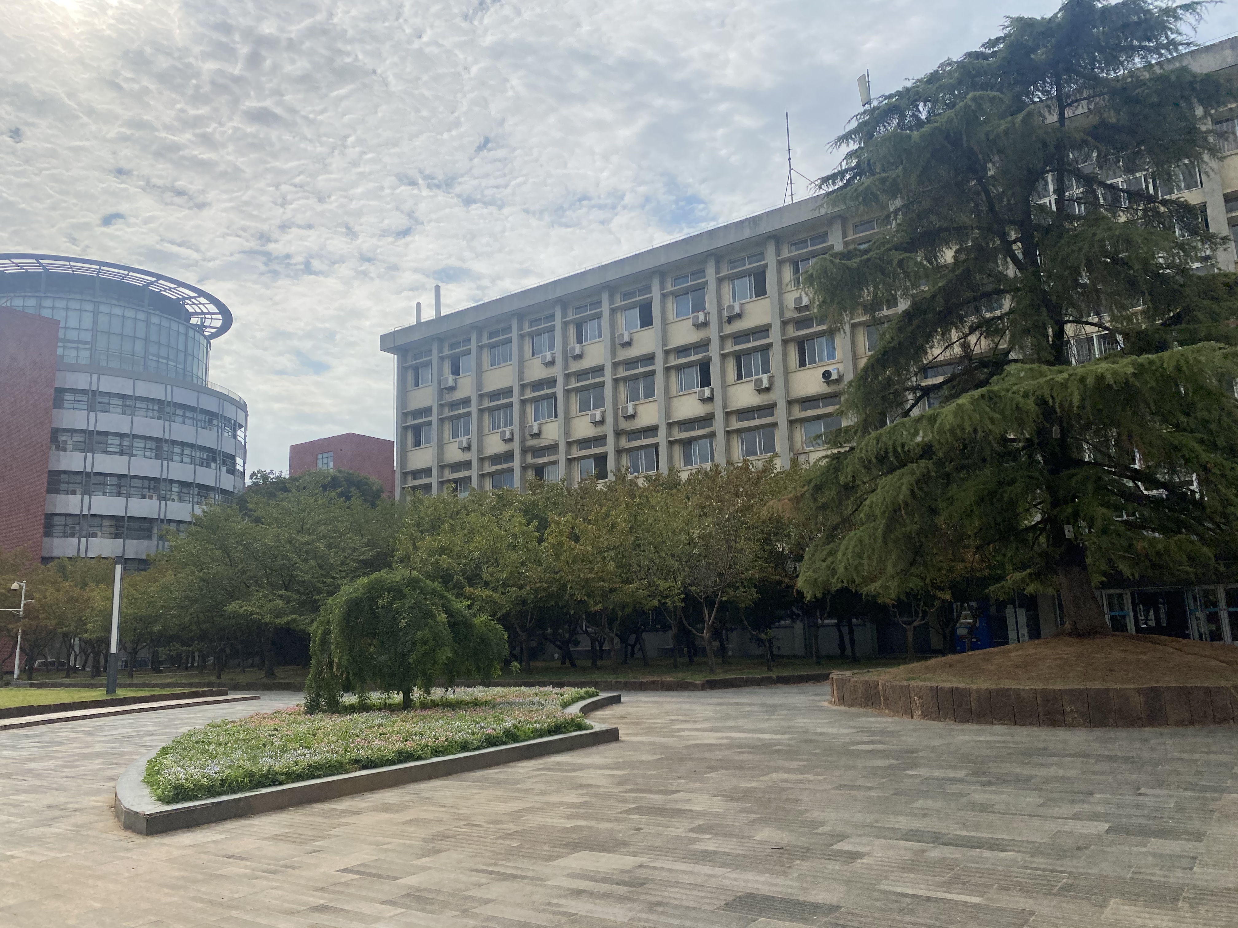
1. imagen original
   
   

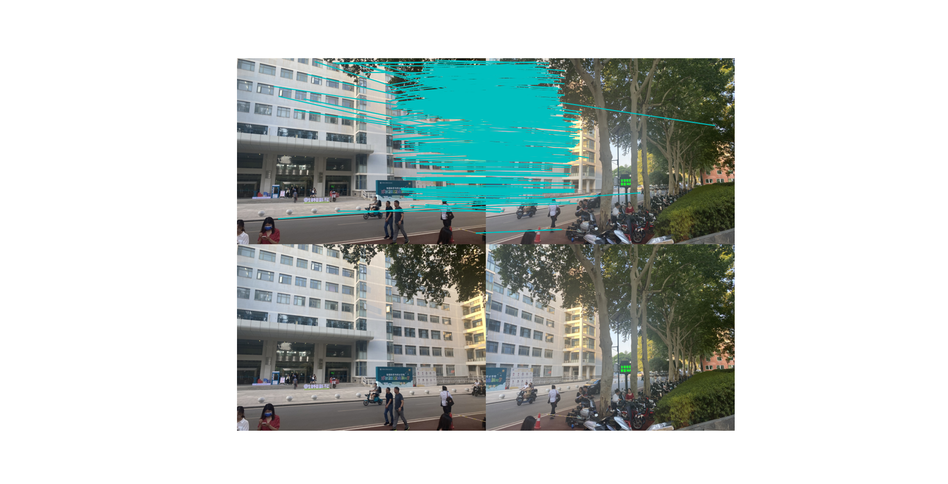
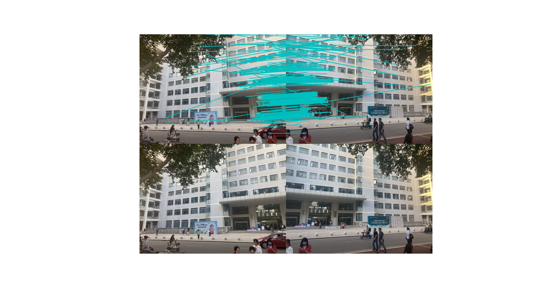
2. característica
   

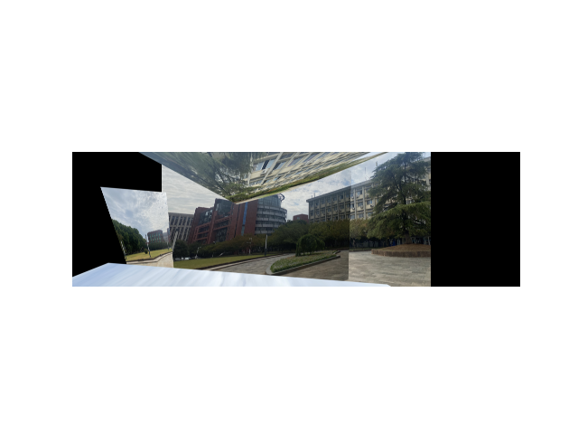
3. Resultados
   
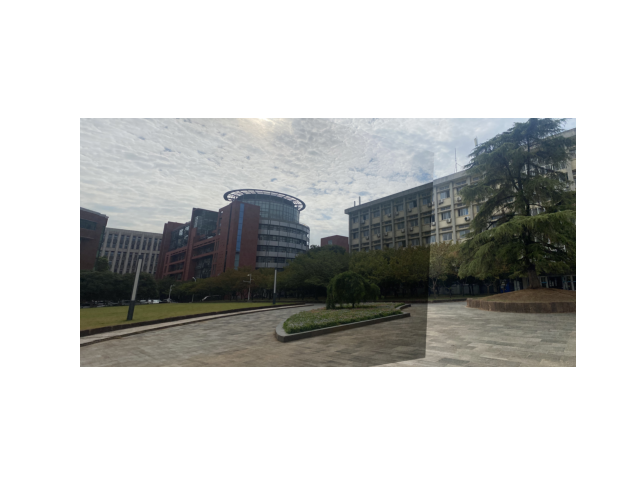
   Hay ciertas diferencias en la profundidad de campo, pero aún se pueden unir imágenes desde diferentes ángulos.

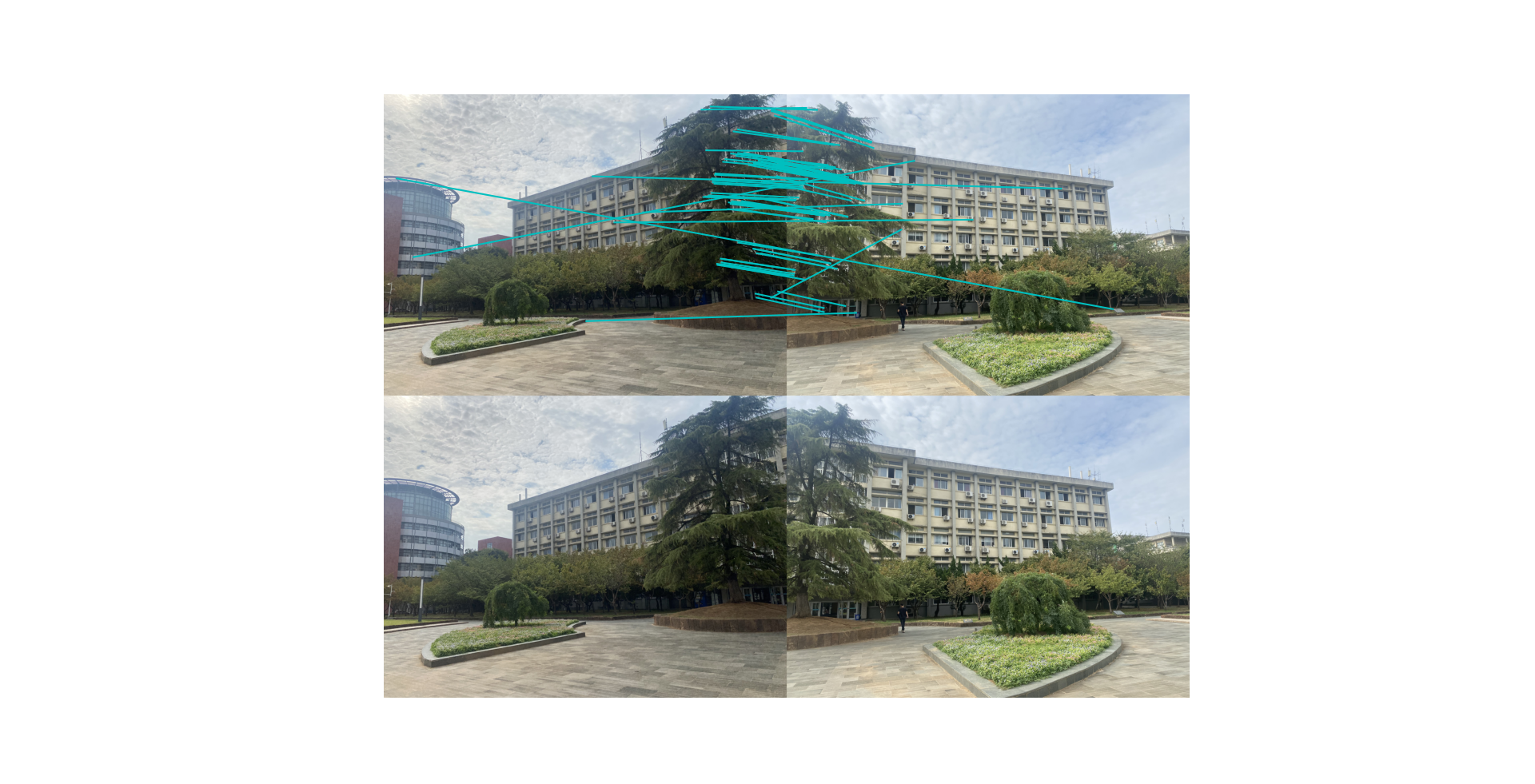
5.3 Unión de tres imágenes

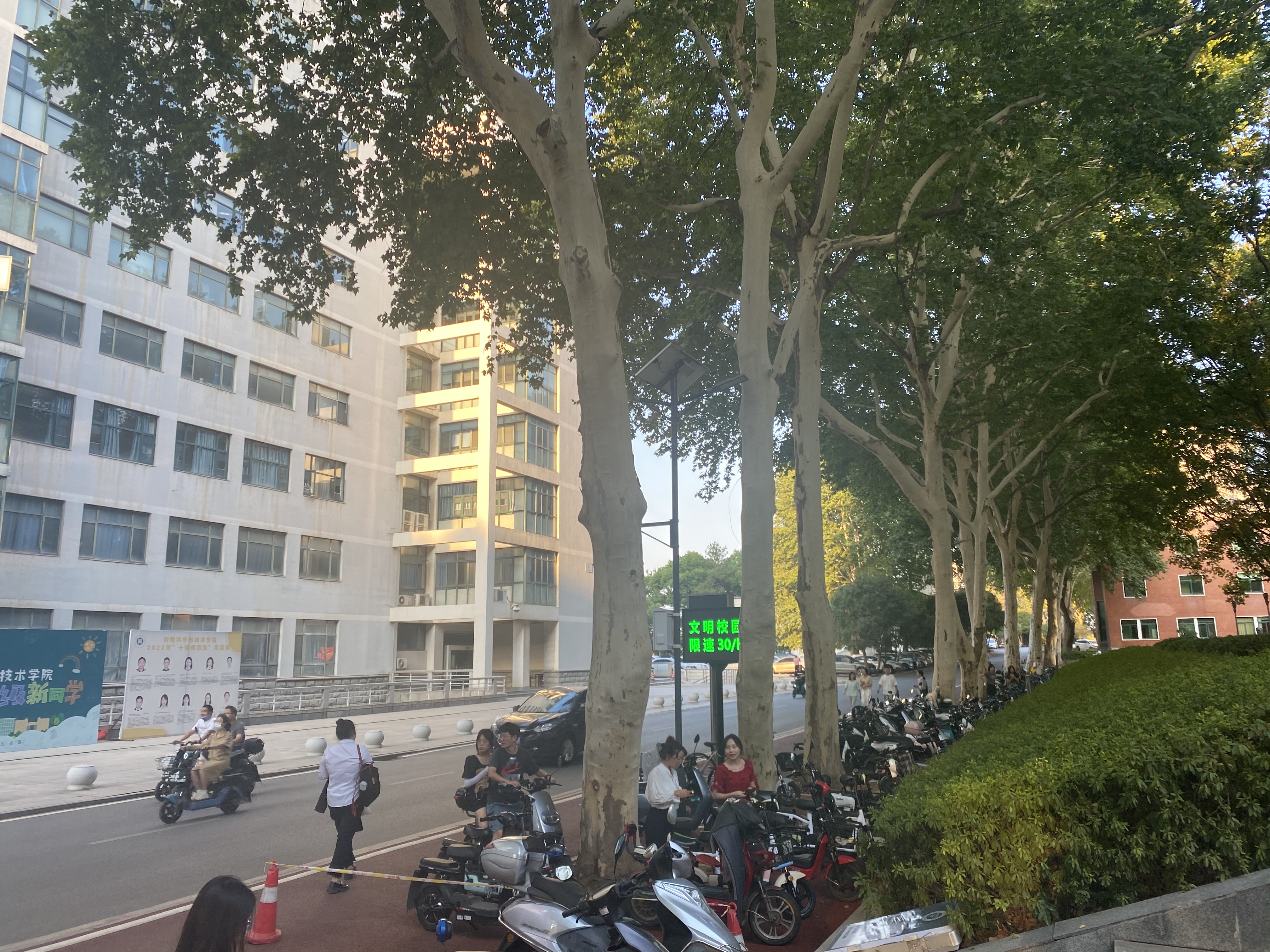
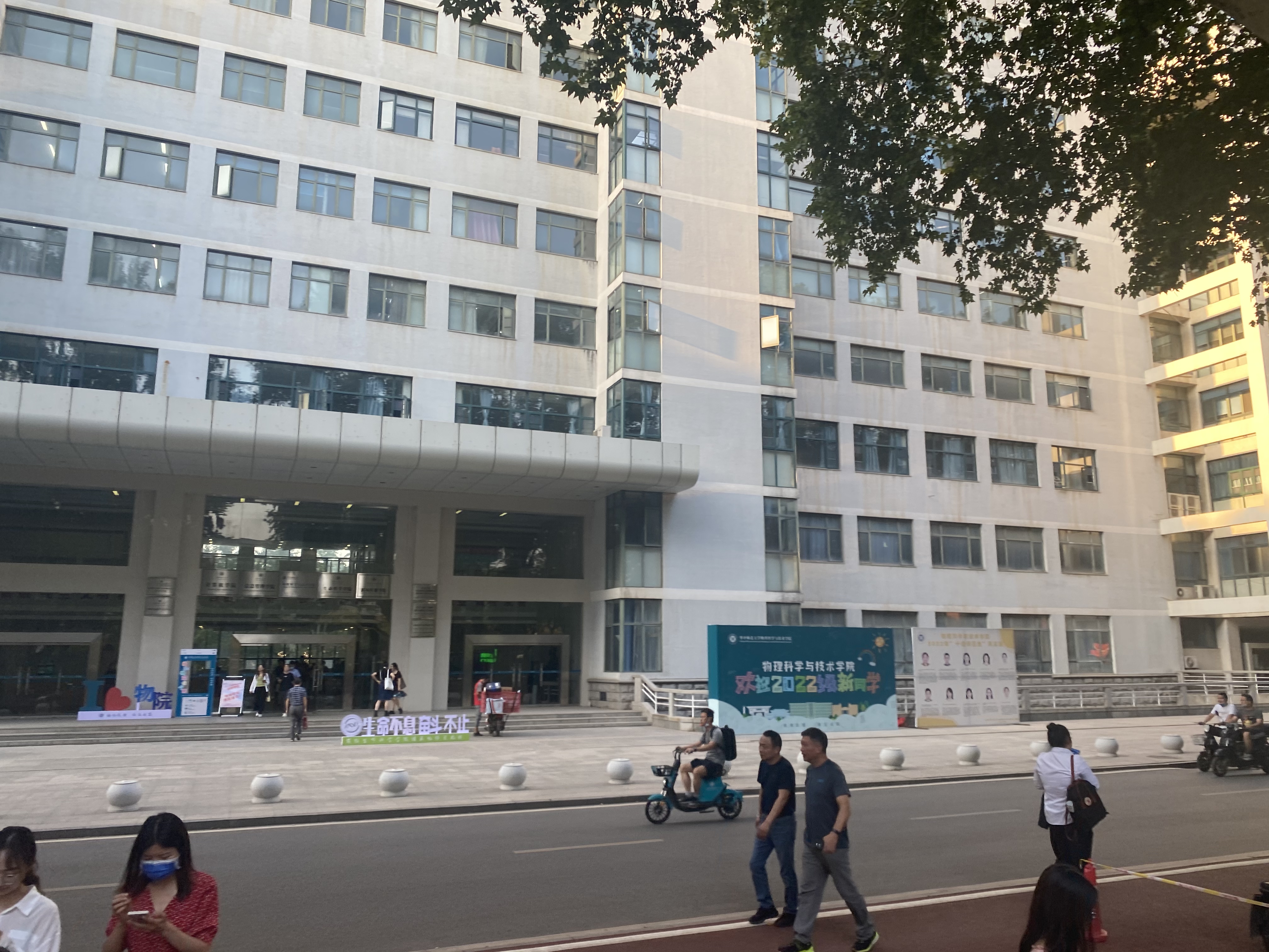
1. imagen original
   
   
   
   

2. característica
   
   

3. resultado de costura
   

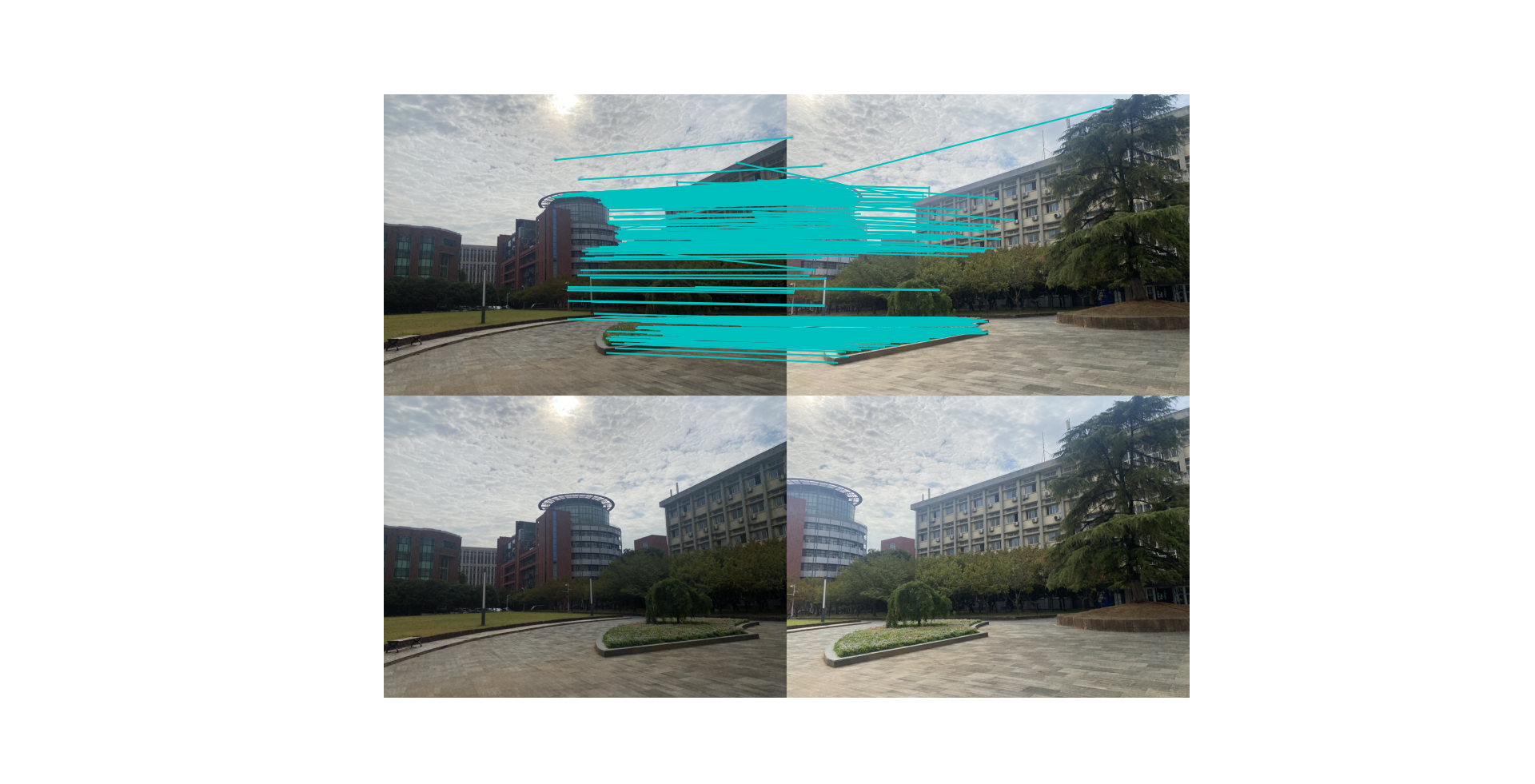
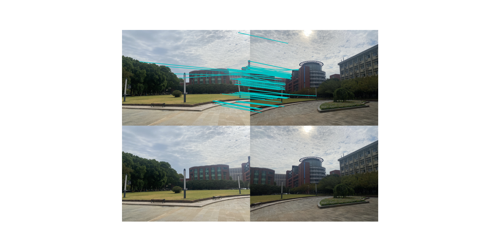
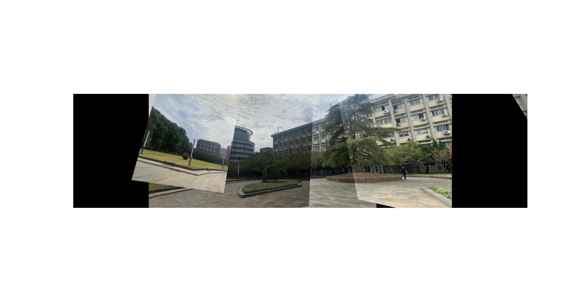
5.4 Unión de cuatro imágenes

1. imagen original
   
   
   
   

2. mapa de características
   
   
   

3. resultado
   

Para el empalme de múltiples imágenes, todavía hay algo de distorsión.

5.5 Unión de cinco imágenes

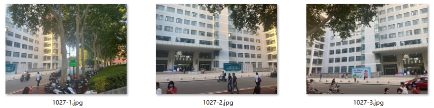
1. Orden de las imágenes originales
   
   
   
   
   
   
   de derecha a izquierda

2. característica
   
   
   
   

3. resultado
   

6. Peinar el proceso de empalme

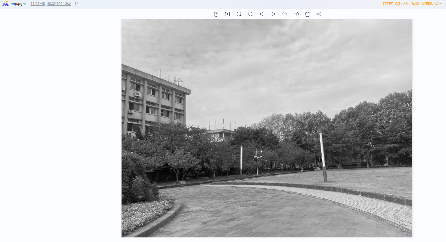
1. Lea el archivo de imagen en la ruta correspondiente y guarde las funciones extraídas en el archivo temporal tmp.pgm
   

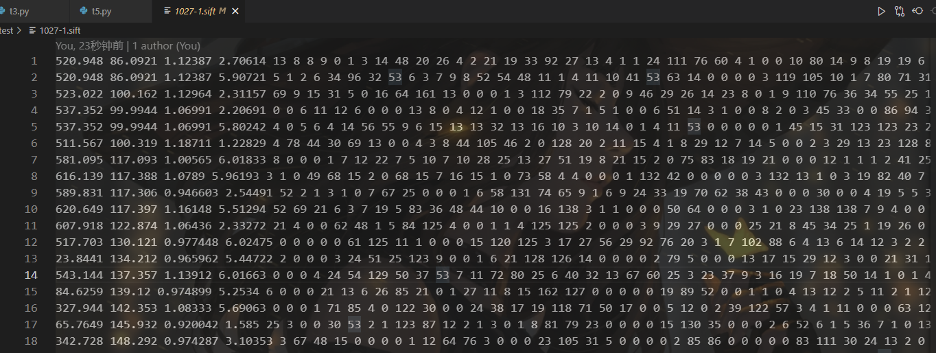
2. La característica se convierte en la matriz de características correspondiente, que se guarda en el archivo .sift
   

3. Haga coincidir las características de las dos imágenes adyacentes respectivamente y visualice la coincidencia de características

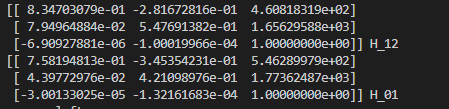
4. Encuentre la matriz de cambio correspondiente a través del método PCV encapsulado y las características combinadas, para realizar la transformación, distorsión y fusión.La
   matriz de transformación correspondiente es la siguiente
   

5. Visualice los resultados de costura
   

apéndice

1. Cambiar dirección de PCV

Basado en el hecho de que los problemas 4 y 5 son causados ​​por la versión de python, subí el código modificado al
código PCV modificado por mí mismo en github

2. Dos códigos de empalme de imágenes

from pylab import *
from numpy import *
from PIL import Image

# If you have PCV installed, these imports should work
from PCV.geometry import homography, warp
from PCV.localdescriptors import sift

"""
This is the panorama example from section 3.3.
"""

# set paths to data folder
# imname使我们要拼接的原图
# featname是sift文件，这个文件是需要根据原图进行生成的
# 需要根据自己的图像地址和图像数量修改地址和循环次数
# featname = ['./images5/'+str(i+1)+'.sift' for i in range(2)] 
# imname = ['./images5/'+str(i+1)+'.jpg' for i in range(2)]
featname = ['./test/1027-'+str(i+1)+'.sift' for i in range(2)] 
imname = ['./test/1027-'+str(i+1)+'.jpg' for i in range(2)]

# extract features and match
l = {
    
    }
d = {
    
    }
for i in range(2): 
    sift.process_image(imname[i],featname[i])
    l[i],d[i] = sift.read_features_from_file(featname[i])

matches = {
    
    }
for i in range(1):
    matches[i] = sift.match(d[i+1],d[i])

# visualize the matches (Figure 3-11 in the book)
for i in range(1):
    im1 = array(Image.open(imname[i]))
    im2 = array(Image.open(imname[i+1]))
    figure()
    sift.plot_matches(im2,im1,l[i+1],l[i],matches[i],show_below=True)


# function to convert the matches to hom. points
def convert_points(j):
    ndx = matches[j].nonzero()[0]
    fp = homography.make_homog(l[j+1][ndx,:2].T) 
    ndx2 = [int(matches[j][i]) for i in ndx]
    tp = homography.make_homog(l[j][ndx2,:2].T) 
    
    # switch x and y - TODO this should move elsewhere
    fp = vstack([fp[1],fp[0],fp[2]])
    tp = vstack([tp[1],tp[0],tp[2]])
    return fp,tp


# estimate the homographies
model = homography.RansacModel() 
# 此代码段为2图图像拼接，若需要多幅图，只需将其中的注释部分取消即可，图像顺序为自右向左。
fp,tp = convert_points(0)
H_01 = homography.H_from_ransac(fp,tp,model)[0] #im 0 to 1

#fp,tp = convert_points(1)
#H_12 = homography.H_from_ransac(fp,tp,model)[0] #im 1 to 2 

#tp,fp = convert_points(2) #NB: reverse order
#H_32 = homography.H_from_ransac(fp,tp,model)[0] #im 3 to 2 

#tp,fp = convert_points(3) #NB: reverse order
#H_43 = homography.H_from_ransac(fp,tp,model)[0] #im 4 to 3    


# warp the images
delta = 2000 # for padding and translation

im1 = array(Image.open(imname[0]), "uint8")
im2 = array(Image.open(imname[1]), "uint8")
im_12 = warp.panorama(H_01,im1,im2,delta,delta)
#im1 = array(Image.open(imname[0]), "f")
#im_02 = warp.panorama(dot(H_12,H_01),im1,im_12,delta,delta)

#im1 = array(Image.open(imname[3]), "f")
#im_32 = warp.panorama(H_32,im1,im_02,delta,delta)

#im1 = array(Image.open(imname[4]), "f")
#im_42 = warp.panorama(dot(H_32,H_43),im1,im_32,delta,2*delta)


figure()
imshow(array(im_12, "uint8"))
axis('off')
savefig("example1.png",dpi=300)
show()

3. Código de empalme de tres imágenes

# 博客方法（三张图）
from pylab import *
from numpy import *
from PIL import Image
 
# If you have PCV installed, these imports should work
from PCV.geometry import homography, warp
from PCV.localdescriptors import sift
np.seterr(invalid='ignore') # 忽略部分警告
"""
This is the panorama example from section 3.3.
"""
 
# 设置数据文件夹的路径
featname = ['test/1027-'+str(i+1)+'.sift' for i in range(3)] 
imname = ['test/1027-'+str(i+1)+'.jpg' for i in range(3)]
 
# 提取特征并匹配使用sift算法
l = {
    
    }
d = {
    
    }
for i in range(3):
    sift.process_image(imname[i], featname[i]) # 处理图像并将结果保存到文件中tmp.pgm，进而保存到.sift文件中
    # feature locations, descriptors要素位置，描述符
    l[i], d[i] = sift.read_features_from_file(featname[i]) # 读取特征属性并以矩阵形式返回
# 特征间两两匹配
matches = {
    
    }
for i in range(2):
    matches[i] = sift.match(d[i + 1], d[i])
 
# 可视化匹配
for i in range(2):
    im1 = array(Image.open(imname[i]))
    im2 = array(Image.open(imname[i + 1]))
    figure()
    # im1、im2（图像作为数组）、locs1、locs2（特征位置）,matchscores（作为“match”的输出），show_below（如果下面应该显示图像）
    sift.plot_matches(im2, im1, l[i + 1], l[i], matches[i], show_below=True)
 
 
# 将匹配转换成齐次坐标点的函数
def convert_points(j):
    ndx = matches[j].nonzero()[0]
    fp = homography.make_homog(l[j + 1][ndx, :2].T)
    ndx2 = [int(matches[j][i]) for i in ndx]
    tp = homography.make_homog(l[j][ndx2, :2].T)
 
    # switch x and y - TODO this should move elsewhere
    fp = vstack([fp[1], fp[0], fp[2]])
    tp = vstack([tp[1], tp[0], tp[2]])
    return fp, tp
 
 
# 估计单应性矩阵
model = homography.RansacModel()
# 博客方法 
fp, tp = convert_points(1)
H_12 = homography.H_from_ransac(fp, tp, model)[0]  # im 1 to 2
print(H_12, 'H_12')
 
fp, tp = convert_points(0)
H_01 = homography.H_from_ransac(fp, tp, model)[0]  # im 0 to 1
print(H_01, 'H_01')
 
# tp, fp = convert_points(2)  # NB: reverse order
# H_32 = homography.H_from_ransac(fp, tp, model)[0]  # im 3 to 2
 
# tp, fp = convert_points(3)  # NB: reverse order
# H_43 = homography.H_from_ransac(fp, tp, model)[0]  # im 4 to 3


 
# 扭曲图像
delta = 1500  # for padding and translation用于填充和平移

# 博客方法
im1 = array(Image.open(imname[1]), "uint8")
im2 = array(Image.open(imname[2]), "uint8")
im_12 = warp.panorama(H_12, im1, im2, delta, delta)

im1 = array(Image.open(imname[0]), "f")
im_02 = warp.panorama(dot(H_12, H_01), im1, im_12, delta, delta)

# im1 = array(Image.open(imname[3]), "f")
# im_32 = warp.panorama(H_32, im1, im_02, delta, delta)

# im1 = array(Image.open(imname[4]), "f")
# im_42 = warp.panorama(dot(H_32, H_43), im1, im_32, delta, 2 * delta)


figure()
imshow(array(im_02, "uint8"))
axis('off')
show()

4. Código de empalme de cuatro imágenes

from pylab import *
from numpy import *
from PIL import Image
 
# If you have PCV installed, these imports should work
from PCV.geometry import homography, warp
from PCV.localdescriptors import sift
np.seterr(invalid='ignore') # 忽略部分警告
"""
This is the panorama example from section 3.3.
"""
 
# 设置数据文件夹的路径
featname = ['test/1027-'+str(i+1)+'.sift' for i in range(4)] 
imname = ['test/1027-'+str(i+1)+'.jpg' for i in range(4)]
 
# 提取特征并匹配使用sift算法
l = {
    
    }
d = {
    
    }
for i in range(4):
    sift.process_image(imname[i], featname[i]) # 处理图像并将结果保存到文件中tmp.pgm，进而保存到.sift文件中
    # feature locations, descriptors要素位置，描述符
    l[i], d[i] = sift.read_features_from_file(featname[i]) # 读取特征属性并以矩阵形式返回
 
matches = {
    
    }
for i in range(3):
    matches[i] = sift.match(d[i + 1], d[i])
 
# 可视化匹配
for i in range(3):
    im1 = array(Image.open(imname[i]))
    im2 = array(Image.open(imname[i + 1]))
    figure()
    # im1、im2（图像作为数组）、locs1、locs2（特征位置）,matchscores（作为“match”的输出），show_below（如果下面应该显示图像）
    sift.plot_matches(im2, im1, l[i + 1], l[i], matches[i], show_below=True)
 
 
# 将匹配转换成齐次坐标点的函数
def convert_points(j):
    ndx = matches[j].nonzero()[0]
    fp = homography.make_homog(l[j + 1][ndx, :2].T)
    ndx2 = [int(matches[j][i]) for i in ndx]
    tp = homography.make_homog(l[j][ndx2, :2].T)
 
    # switch x and y - TODO this should move elsewhere
    fp = vstack([fp[1], fp[0], fp[2]])
    tp = vstack([tp[1], tp[0], tp[2]])
    return fp, tp
 
 
# 估计单应性矩阵
model = homography.RansacModel()
# 博客方法 
fp, tp = convert_points(1)
H_12 = homography.H_from_ransac(fp, tp, model)[0]  # im 1 to 2
 
fp, tp = convert_points(0)
H_01 = homography.H_from_ransac(fp, tp, model)[0]  # im 0 to 1
 
tp, fp = convert_points(2)  # NB: reverse order
H_32 = homography.H_from_ransac(fp, tp, model)[0]  # im 3 to 2
 
# tp, fp = convert_points(3)  # NB: reverse order
# H_43 = homography.H_from_ransac(fp, tp, model)[0]  # im 4 to 3

 
# 扭曲图像
delta = 2000  # for padding and translation用于填充和平移

# 博客方法
im1 = array(Image.open(imname[1]), "uint8")
im2 = array(Image.open(imname[2]), "uint8")
im_12 = warp.panorama(H_12, im1, im2, delta, delta)
 
im1 = array(Image.open(imname[0]), "f")
im_02 = warp.panorama(dot(H_12, H_01), im1, im_12, delta, delta)
 
im1 = array(Image.open(imname[3]), "f")
im_32 = warp.panorama(H_32, im1, im_02, delta, delta)
 
# im1 = array(Image.open(imname[4]), "f")
# im_42 = warp.panorama(dot(H_32, H_43), im1, im_32, delta, 2 * delta)



figure()
imshow(array(im_32, "uint8"))
axis('off')
show()

5. Cinco códigos de empalme de imágenes

# -*- codeing =utf-8 -*-
# @Time : 2021/4/20 11:00
# @Author : ArLin
# @File : demo1.py
# @Software: PyCharm
from pylab import *
from numpy import *
from PIL import Image

# If you have PCV installed, these imports should work
from PCV.geometry import homography, warp
from PCV.localdescriptors import sift
np.seterr(invalid='ignore')
"""
This is the panorama example from section 3.3.
"""

# 设置数据文件夹的路径
featname = ['./test/1027-'+str(i+1)+'.sift' for i in range(5)] 
imname = ['./test/1027-'+str(i+1)+'.jpg' for i in range(5)]

# 提取特征并匹配使用sift算法
l = {
    
    }
d = {
    
    }
for i in range(5):
    sift.process_image(imname[i], featname[i])
    l[i], d[i] = sift.read_features_from_file(featname[i])

matches = {
    
    }
for i in range(4):
    matches[i] = sift.match(d[i + 1], d[i])

# 可视化匹配
for i in range(4):
    im1 = array(Image.open(imname[i]))
    im2 = array(Image.open(imname[i + 1]))
    figure()
    sift.plot_matches(im2, im1, l[i + 1], l[i], matches[i], show_below=True)


# 将匹配转换成齐次坐标点的函数
def convert_points(j):
    ndx = matches[j].nonzero()[0]
    fp = homography.make_homog(l[j + 1][ndx, :2].T)
    ndx2 = [int(matches[j][i]) for i in ndx]
    tp = homography.make_homog(l[j][ndx2, :2].T)

    # switch x and y - TODO this should move elsewhere
    fp = vstack([fp[1], fp[0], fp[2]])
    tp = vstack([tp[1], tp[0], tp[2]])
    return fp, tp


# 估计单应性矩阵
model = homography.RansacModel()

fp, tp = convert_points(1)
H_12 = homography.H_from_ransac(fp, tp, model)[0]  # im 1 to 2

fp, tp = convert_points(0)
H_01 = homography.H_from_ransac(fp, tp, model)[0]  # im 0 to 1

tp, fp = convert_points(2)  # NB: reverse order
H_32 = homography.H_from_ransac(fp, tp, model)[0]  # im 3 to 2

tp, fp = convert_points(3)  # NB: reverse order
H_43 = homography.H_from_ransac(fp, tp, model)[0]  # im 4 to 3

# 扭曲图像
delta = 2000  # for padding and translation用于填充和平移

im1 = array(Image.open(imname[1]), "uint8")
im2 = array(Image.open(imname[2]), "uint8")
im_12 = warp.panorama(H_12, im1, im2, delta, delta)

im1 = array(Image.open(imname[0]), "f")
im_02 = warp.panorama(dot(H_12, H_01), im1, im_12, delta, delta)

im1 = array(Image.open(imname[3]), "f")
im_32 = warp.panorama(H_32, im1, im_02, delta, delta)

im1 = array(Image.open(imname[4]), "f")
im_42 = warp.panorama(dot(H_32, H_43), im1, im_32, delta, 2 * delta)

figure()
imshow(array(im_42, "uint8"))
axis('off')
show()