A better optimization method
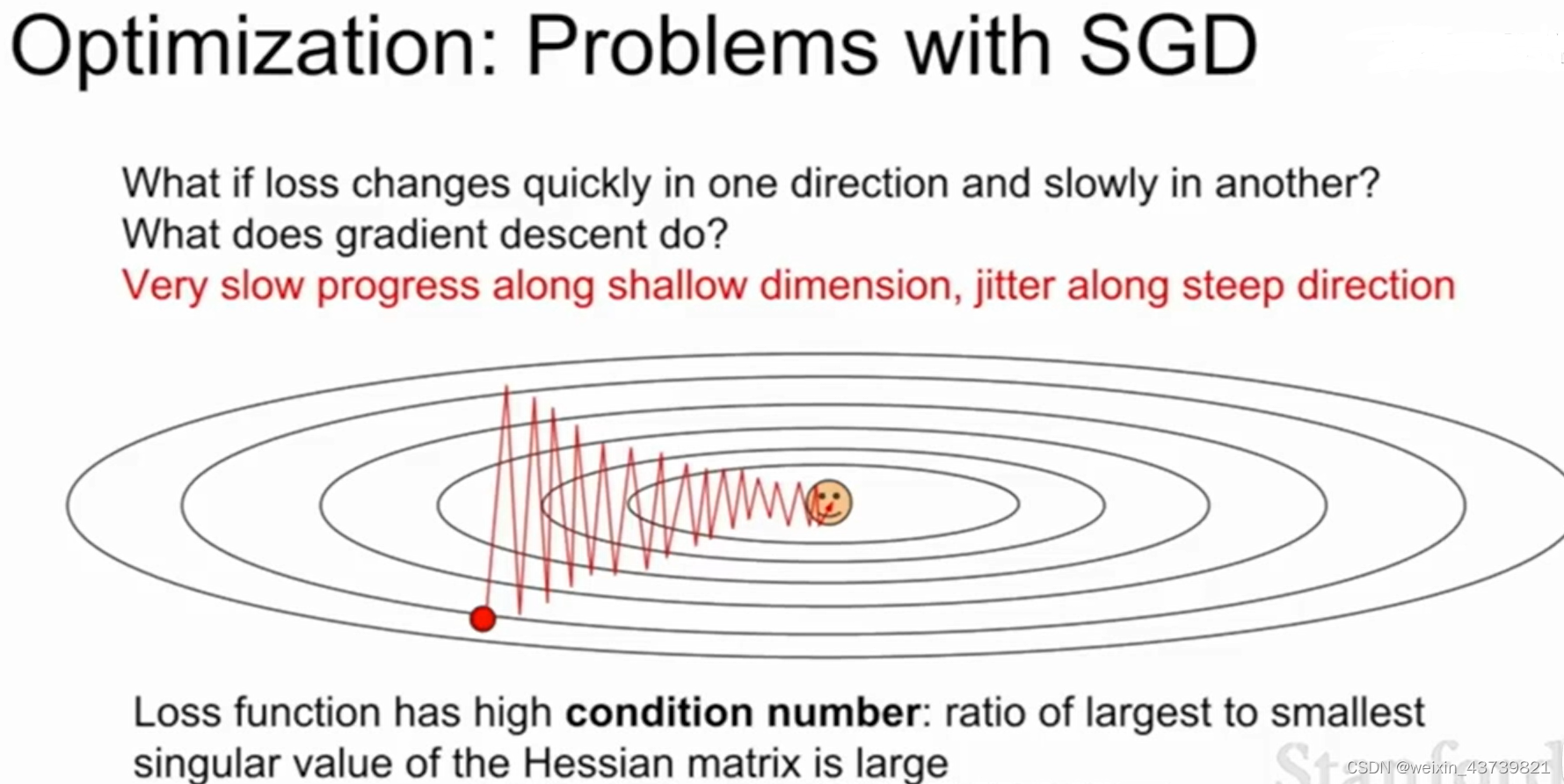
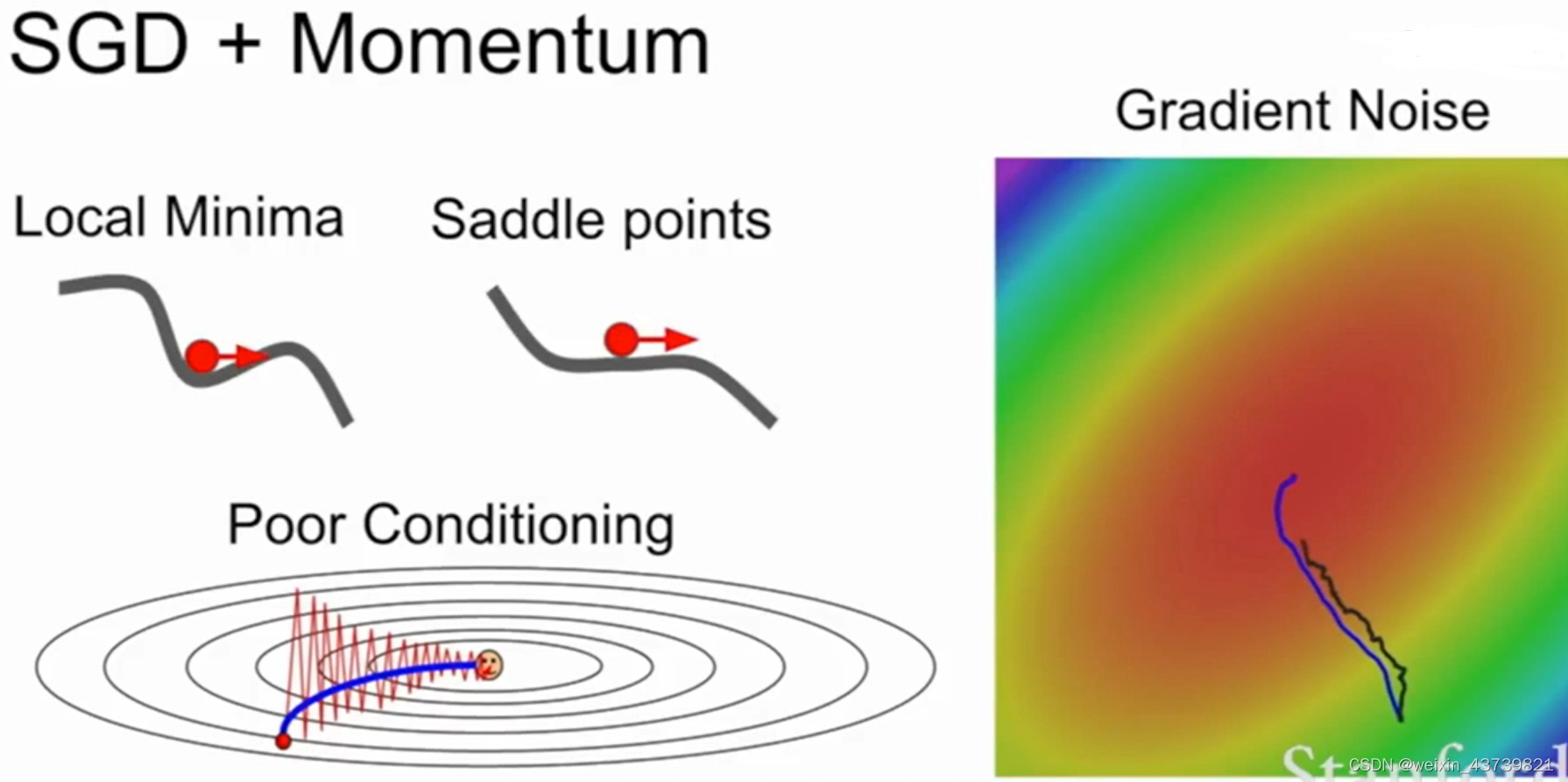
The stochastic gradient descent (SGD) mentioned above will cause many problems in actual use. For example, the loss function in the figure below is not sensitive to the horizontal direction but sensitive to the vertical direction. In fact, in higher dimensions This problem is more pronounced when very many parameters are involved.
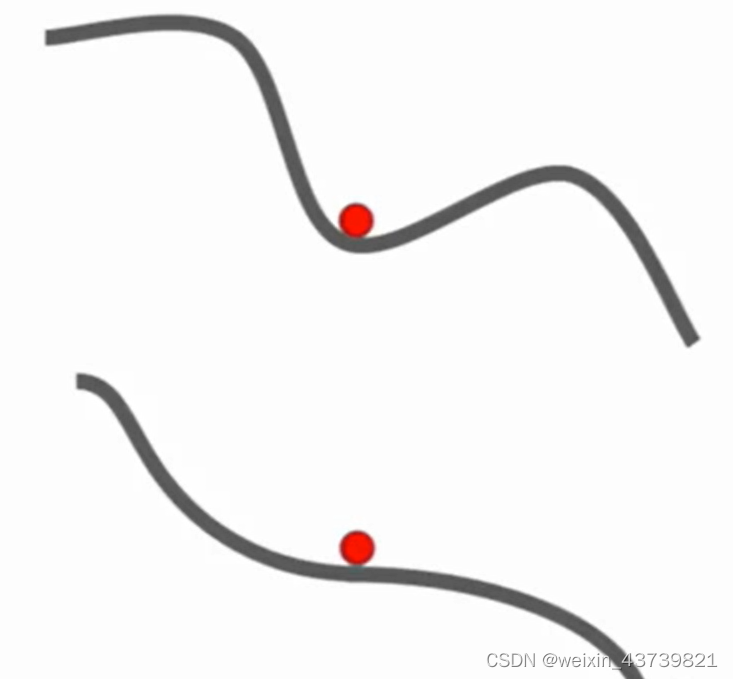
Another problem is the local minimum or saddle point. As shown in the figure below, the X-axis is the value of the parameter, and the Y-axis is the loss value. SGD may fall into a local optimum or a saddle point. At that point, the gradient value is 0 or close to 0. So Does not move or is very slow.
Another problem is that each step of stochastic gradient descent estimates the loss and gradient through a small batch of examples, so if there is noise in the gradient estimation, it will actually take a long time.
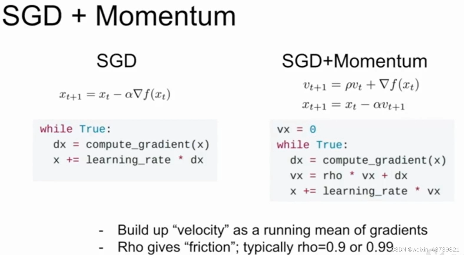
A very simple strategy to solve this problem is to add a momentum term to stochastic gradient descent. As shown on the right side of the figure, there is a very small variance, which is called SGD with momentum . The idea is to add inertia/speed so that the optimization is not easy to fall into the local optimum or stay at the saddle point. Each step uses the friction coefficient ρ (taken The value is generally large, such as 0.9) to attenuate the speed and then add it to the gradient to maintain a speed that does not change over time, and we add the gradient estimate to this speed, and then step in the direction of this speed instead of in the gradient step in the direction of . It is such a super simple idea that solves all the above problems
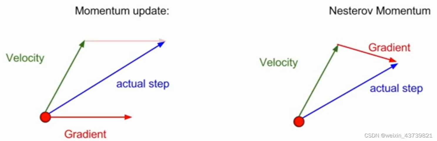
There is also a change in the form of momentum called Nesterov acceleration gradient, or Nesterov momentum, which is different from the current actual direction obtained by mixing the speed and the current gradient before, but steps in the direction of the speed at the red point, and then evaluates the step. The gradient of the position, and then return to the initial test position to mix the two. This "forward-looking" method can reach the optimal point faster. This also has some nice theoretical properties for convex optimization problems, but has some problems when it comes to non-convex optimization problems such as neural networks.
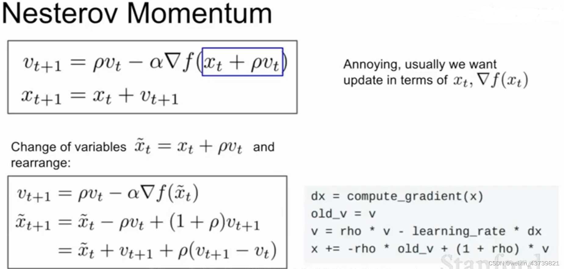
Nesterov's formula is a bit inconvenient, because when using SGD optimization, it is generally desired to calculate the loss function and gradient at the same time, and its formula will cause damage to this and cause trouble in application. Fortunately, we can use the substitution method to improve the Nestero formula to replace variables , can be calculated simultaneously.
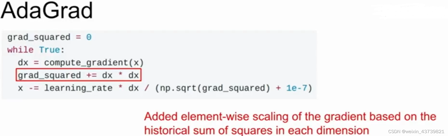
Another common optimization strategy is the AdaGrad algorithm . The core idea is to maintain a continuous estimate of the sum of the squares of the gradients at each step in the training process during the optimization process. Now there is a gradient squared item, and it will always be during training. Accumulate the current gradient squared to this gradient squared term, which is divided by the gradient squared term when we update the parameter vector (add 1e-7 to prevent dividing by 0). So what is the improvement of such scaling for the case where the condition number in the matrix is large?
Taking the previous example, if we have two axes and we have a high gradient along one axis and a small gradient along the other, then as we accumulate the square of the small gradient, we divide by a small The number thus accelerates the learning speed in small gradient dimensions, and the opposite is true for high dimensions. So what happens as the square term gets bigger and bigger over time?
It will make the step size smaller and smaller, so when the objective function is a convex function, the training effect is better, but it is not good under a non-convex function, and it is easy to fall into a local optimum. This algorithm is generally not recommended when doing neural network training.
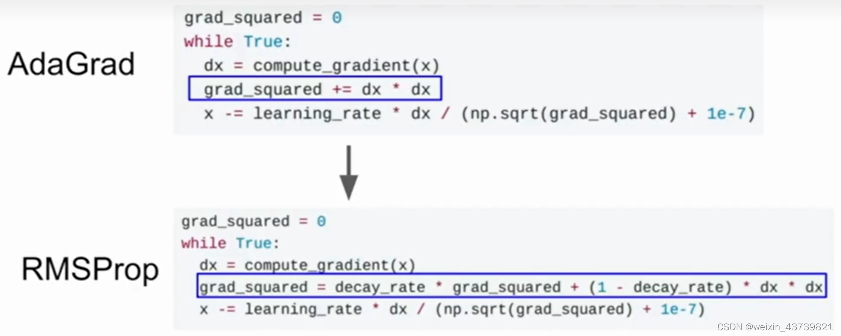
For the defects of AdaGrad, there is a variant of AdaGrad called RMSProp that takes this problem into account. It still calculates the squared gradients, but instead of just accumulating the squared gradients during training, it lets the squared gradients fall off at a certain rate so that it looks a lot like momentum optimization, except we add momentum to the squared gradients instead of to the gradient itself.
With RMSProp, after calculating the gradient, take out the current gradient square item and multiply it by a decay rate, usually 0.9 or 0.99, and then subtract the decay rate from 1 by the gradient square and add them. This still retains the advantages of AdaGrad with different gradients on different axes but maintaining the learning speed.
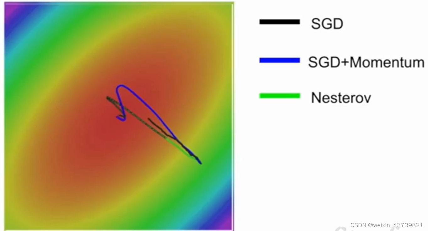
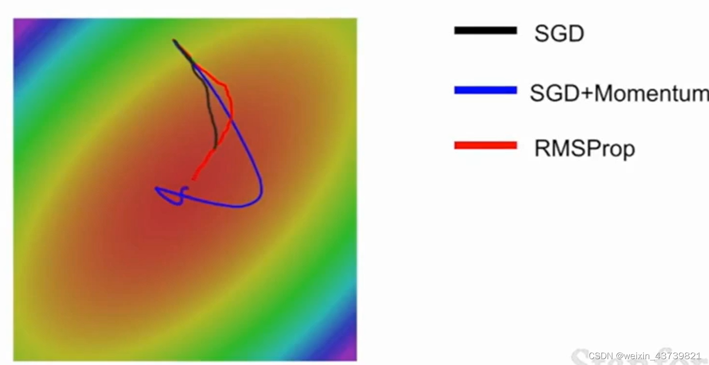
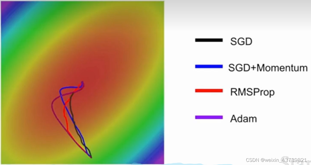
It can be seen that the effect of RMSProp and SGD with momentum is better than that of pure SGD, but SGD with momentum will first bypass the minimum value and then turn back. RMSProp has been adjusting its route, which is to make roughly the same optimization.
The above two methods, one is the concept of speed along the direction of the speed, the other is the concept of gradient square, both of these methods look good, so they can also be combined, which is the famous Adam algorithm .
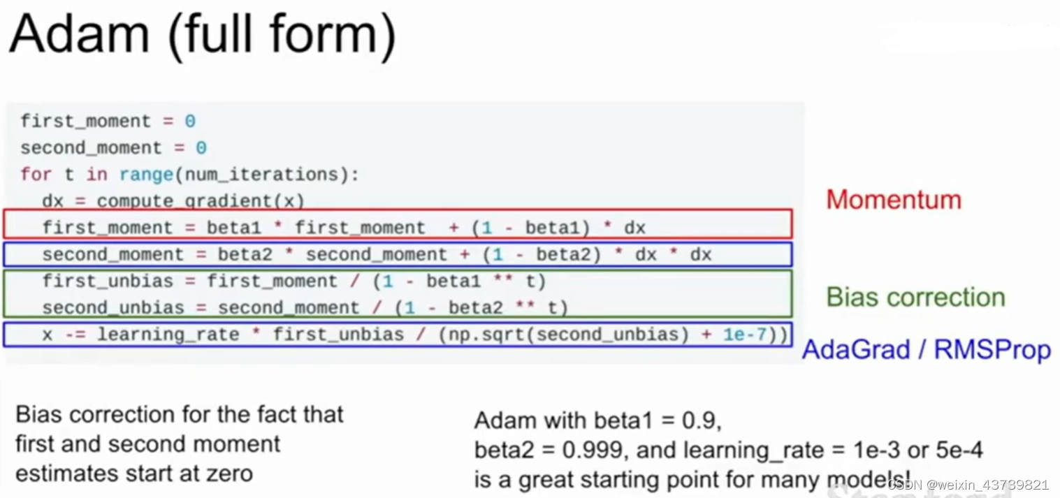
Using Adam, we update the estimated value of the first momentum and the second momentum. In the red box below, we make the estimated value of the first momentum equal to the weighted sum of our gradients. The estimated value of the second momentum is a gradient square like AdaGrad and RMSProp A dynamic approximation of . We use the first momentum a bit like velocity and divide by the second momentum or the square root of the second momentum, so Adam is a bit like AdaGrad plus momentum or looks like momentum plus the second gradient squared, combining the advantages of both .
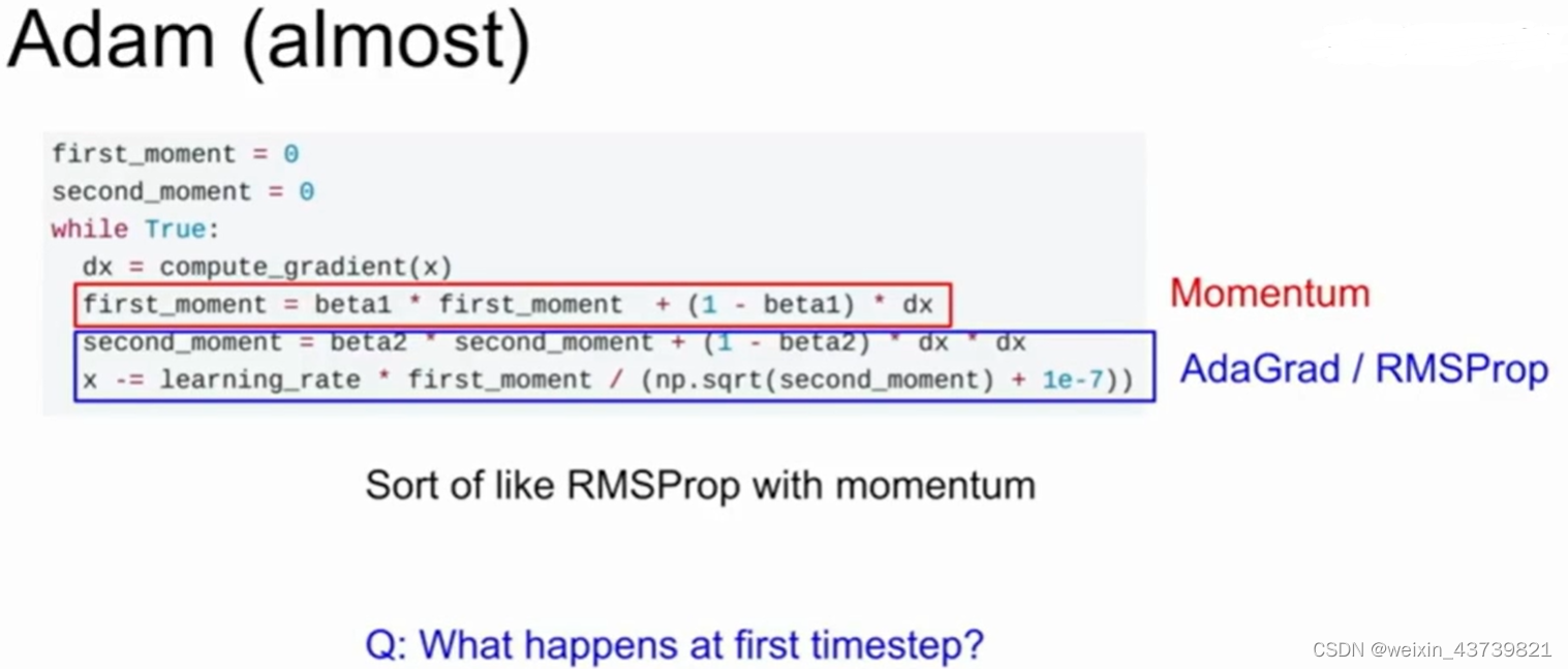
But there is still a problem. When the first few steps are updated, because the second momentum is initialized to 0, it is very small, so it may get a large step size and mess things up, so the Adam algorithm also adds a bias correction item to avoid this problem. By using the current time step t, we construct the unbiased estimates of the first and second momentums, and use the unbiased estimates to update each step. This is the complete form of Adam. Generally, the first consideration for solving any problem is the Adam algorithm. , especially set beta1 to 0.9, beta2 to 0.999, and the learning rate to 1e-3 or 5e-4. No matter what network architecture is used, it will start from this setting.
Learning rate selection skills
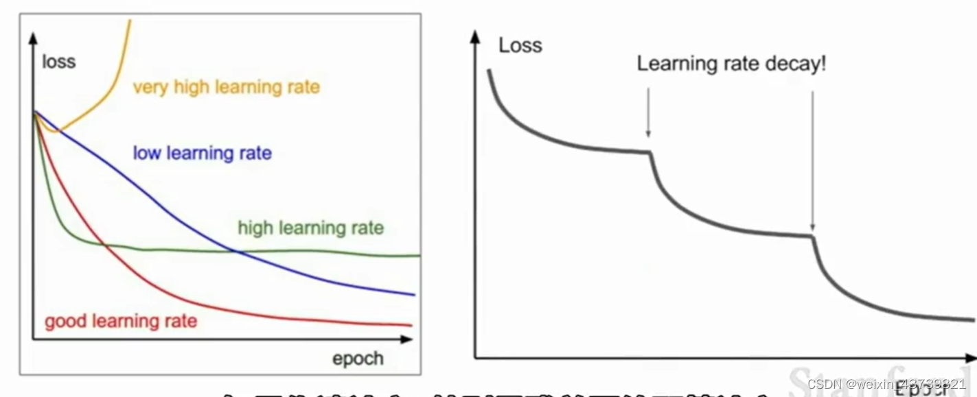
We don't have to use the same learning rate throughout the training process. Sometimes people will decay the learning rate along time, which is a bit like combining the effects of different curves in the left picture, and it is in each picture nice nature. For example, use a larger learning rate at the beginning, and then gradually decrease it during the training process.
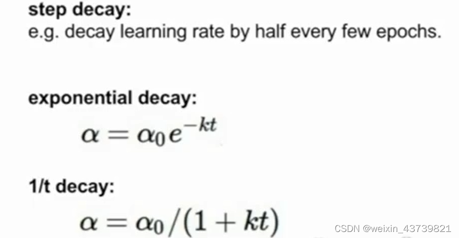
One strategy is step decay, for example, at the 100,000th iteration, you can decay by a factor and then continue training; there is also exponential decay, which is continuous decay during training.
If you read papers, especially those on residual networks, you will often see such curves. Behind such a curve is actually the learning rate with step size decay. The sudden drop is that the learning rate is multiplied by a decay during iteration. Factor, the idea is that the model is already close to a good value area and the gradient is already very small. Keeping the original learning rate can only hover around the optimal point, but reducing the objective function can still be further optimized.
TIPS: The learning rate decay of SGD with momentum is very common, but optimization algorithms like Adam are rarely used. Another point to point out is that you should not use the learning rate decay from the beginning. You need to choose a good fixed learning rate at the beginning. Trying to adjust the learning rate decay and the initial learning rate in the cross-validation will be confusing. You should try it first. Decay to see what happens and watch the loss curve carefully to see where you expect the decay to start.
TIPS: What I mentioned earlier is to reduce the training error, but how to reduce the error gap between training and testing?
A quick, clumsy and easy way is model ensemble, instead of using one model we choose to train 10 different models from different random initial values, when it comes time to test we run the test data on 10 models and then evaluate 10 models Adding these models together can alleviate some overfitting and improve some performance, usually a few percentage points, not a big but fixed improvement.
Sometimes the hyperparameters are not the same during ensemble learning. You may try models of different sizes, different learning rates, and different regularization strategies, and then put them together for ensemble learning.
With a little more creativity, sometimes instead of training different models independently, you can keep snapshots of multiple models during the training process, and then use these models for ensemble learning, and then combine these multiple snapshots during the test phase. The prediction results are averaged.
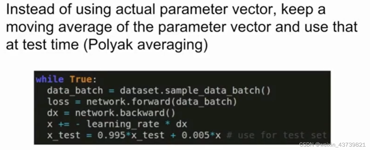
TIPS: Another trick that may be used is to calculate the exponential decay average value of each model parameter at different times when training the model, so as to obtain a relatively smooth integrated model in network training, and then use these smooth decay averages Model parameters, rather than model parameters that end at a certain moment, this is called Polyak averaging, which may sometimes have some effects but is not common.
Regularization
In addition to ensemble learning, we hope to find an effect that can improve a single model. Regularization is, we have introduced some before, such as L2 regularization.
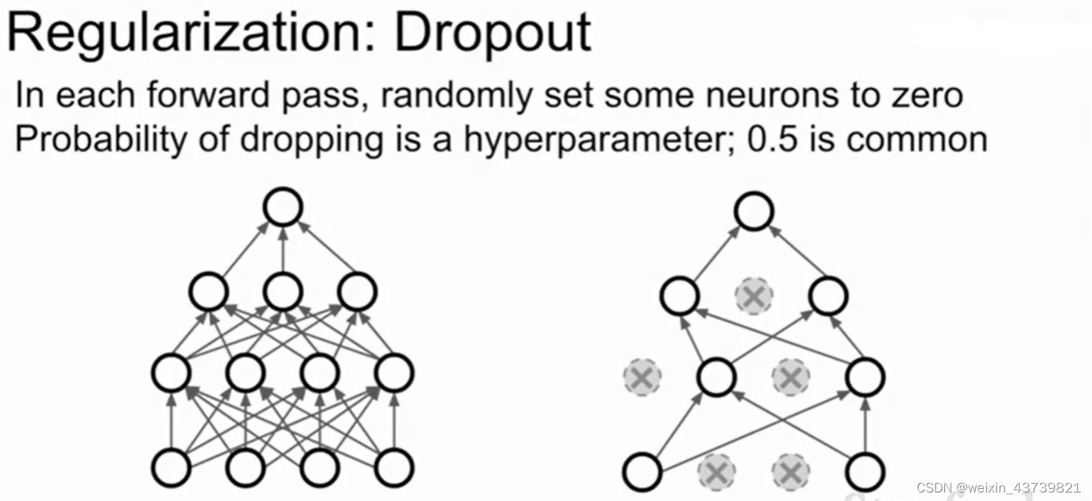
A particularly commonly used method in neural networks is dropout, which is very simple. Every time it propagates forward in the network, it randomly sets a part of neurons to 0 in each layer (set the value of the activation function to 0, and each layer It is to calculate the result of the previous activation function multiplied by the weight matrix, then the input of the activation function of the next layer will be partly 0), and the neurons that are randomly set to 0 in each forward pass are not exactly the same.
In the neural network, dropout is generally used in the fully connected layer, and in the convolutional neural network, a certain feature is randomly mapped to the entire intelligence 0.

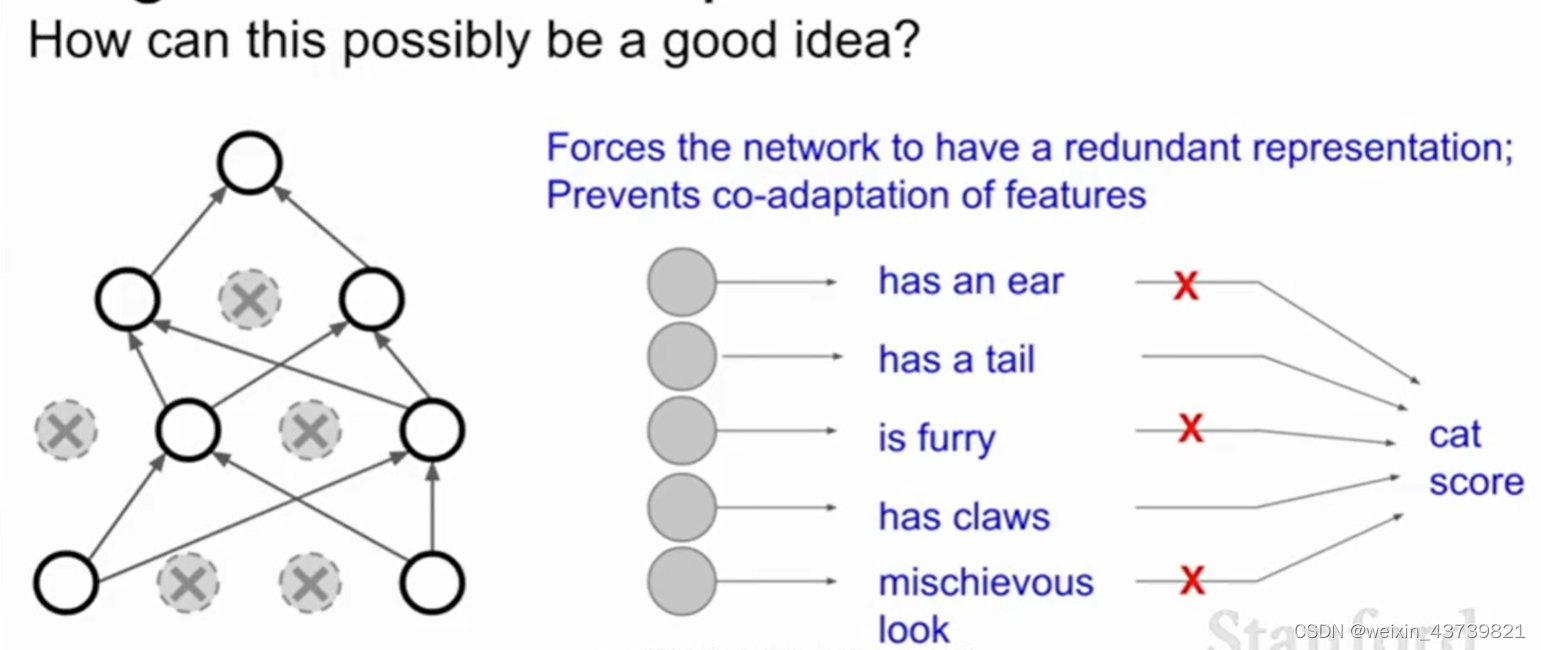
Why does this make sense? People think that this avoids mutual adaptation between features. Suppose we want to classify and judge whether it is a cat. Maybe one neuron in the network has learned that it has an ear, one has learned a tail, and one has learned that there is a cat. hair, and then these features are combined to determine whether it is a cat or not. However, after adding dropout to judge whether it is a cat, the network cannot rely on the results given by the combination of these features, but must use different scattered features to judge, which suppresses overfitting to some extent.
Another explanation about dropout is that it is an integrated learning in a single model, because looking at the left picture, after dropout, it is operated in a sub-network, and each possible dropout method produces a different sub-network, so dropout It is like performing ensemble learning on a group of networks sharing parameters at the same time.
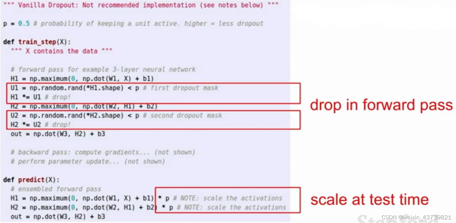
Because of the randomness of dropout, we have difficulties in testing. Each training step will create an independent neural network, because each nerve may appear or not, so there are a total of 2 to the Nth power possible network (N is the number of neurons that can be discarded), and it is completely impossible to test so many subnets and then take the average during testing, and dropout cannot be turned off during testing. Dropout is added during training to prevent overfitting , which is a completely different model if it is turned off during testing. But if the dropout is not turned off, the result y may be random, so in order to make the test without any randomness, we return the probability of dropout multiplied by the output to get the same expected value output, because each neuron has p probability is discarded.
To sum up, dropout is very simple in forward propagation, you only need to add two lines to the implementation, and randomly set some nodes to 0. Then add a little multiplication to your probabilities inside the predict function at test time.