Analysis of the distribution and distribution type distribution → research data, quantitative data points, the amount of basic statistics to distinguish qualitative data
AS NP numpy Import
Import PANDAS AS PD
Import matplotlib.pyplot AS PLT
% matplotlib inline
# data reading data = pd.read_csv ( 'C: / Users / 83759 / Desktop / hand housing Luohu information .csv', engine = ' Python ') plt.scatter (Data [' Lon '], Data [' latitude '], in accordance with the latitude and longitude display #           s = data [' Housing Unit '] / 500, in accordance with monovalent display size #           c = data [' reference total '], in accordance with the total display color #           Alpha = 0.4, CMap =' Reds')   plt.grid () Print (data.dtypes) Print ( '------- \% i n-pieces of data length'% len (data)) data.head () # can be seen by the data, a total of eight fields # quantitative fields: Housing Unit, reference down, the reference price, * longitude, latitude *, * house code # qualitative fields: cell, towards

Range: max-min
Only for quantitative field
def d_range(df,*cols):
krange = []
for col in cols:
crange = df[col].max() - df[col].min()
krange.append(crange)
return(krange)
# 创建函数求极差
key1 = '参考首付'
key2 = '参考总价'
dr = d_range(data,key1,key2)
print('%s极差为 %f \n%s极差为 %f' % (key1, dr[0], key2, dr[1]))
# 求出数据对应列的极差

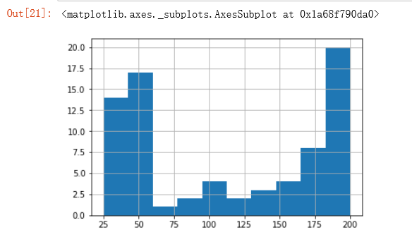
频率分布情况 - 定量字段
① 通过直方图直接判断分组组数
简单查看数据分布,确定分布组数 → 一般8-16即可,这里以10组为参考
data[key2].hist(bins=10)
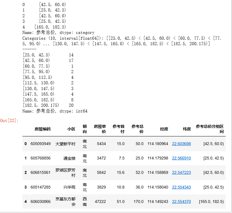
② 求出分组区间
pd.cut(x, bins, right):按照组数对x分组,且返回一个和x同样长度的分组dataframe,right → 是否右边包含,默认True
通过groupby查看不同组的数据频率分布
给源数据data添加“分组区间”列
gcut = pd.cut(data[key2],10,right=False)
gcut_count = gcut.value_counts(sort=False) # 不排序
data['%s分组区间' % key2] = gcut.values
print(gcut.head(),'\n------')
print(gcut_count)
data.head()
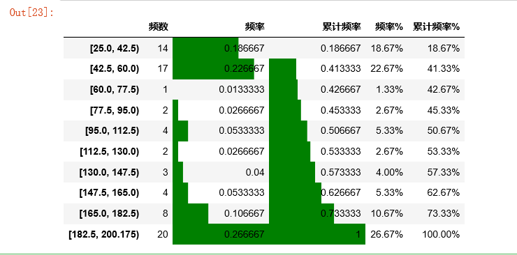
③ 求出目标字段下频率分布的其他统计量 → 频数,频率,累计频率
r_zj = pd.DataFrame(gcut_count)
r_zj.rename(columns ={gcut_count.name:'频数'}, inplace = True) # 修改频数字段名
r_zj['频率'] = r_zj / r_zj['频数'].sum() # 计算频率
r_zj['累计频率'] = r_zj['频率'].cumsum() # 计算累计频率
r_zj['频率%'] = r_zj['频率'].apply(lambda x: "%.2f%%" % (x*100)) # 以百分比显示频率
r_zj['累计频率%'] = r_zj['累计频率'].apply(lambda x: "%.2f%%" % (x*100)) # 以百分比显示累计频率
r_zj.style.bar(subset=['频率','累计频率'], color='green',width=100)
④ 绘制频率直方图
r_zj['频率'].plot(kind = 'bar',
width = 0.8,
figsize = (12,2),
rot = 0,
color = 'k',
grid = True,
alpha = 0.5)
plt.title('参考总价分布频率直方图')
# 绘制直方图
x = len(r_zj)
y = r_zj['频率']
m = r_zj['频数']
for i,j,k in zip(range(x),y,m):
plt.text(i-0.1,j+0.01,'%i' % k, color = 'k')
# 添加频数标签

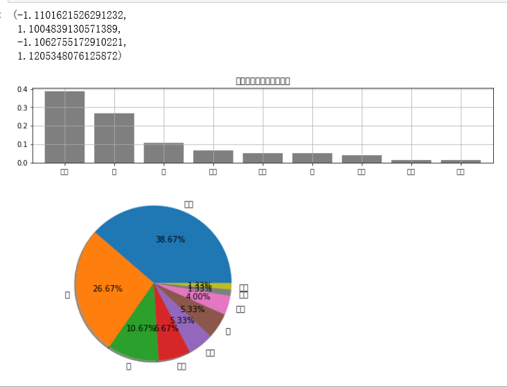
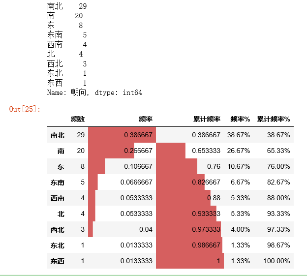
频率分布情况 - 定性字段
① 通过计数统计判断不同类别的频率
cx_g = data['朝向'].value_counts(sort=True)
print(cx_g)
# 统计频率
r_cx = pd.DataFrame(cx_g)
r_cx.rename(columns ={cx_g.name:'频数'}, inplace = True) # 修改频数字段名
r_cx['频率'] = r_cx / r_cx['频数'].sum() # 计算频率
r_cx['累计频率'] = r_cx['频率'].cumsum() # 计算累计频率
r_cx['频率%'] = r_cx['频率'].apply(lambda x: "%.2f%%" % (x*100)) # 以百分比显示频率
r_cx['累计频率%'] = r_cx['累计频率'].apply(lambda x: "%.2f%%" % (x*100)) # 以百分比显示累计频率
r_cx.style.bar(subset=['频率','累计频率'], color='#d65f5f',width=100)
# 可视化显示

② 绘制频率直方图、饼图
plt.figure(num = 1,figsize = (12,2))
r_cx['频率'].plot(kind = 'bar',
width = 0.8,
rot = 0,
color = 'k',
grid = True,
alpha = 0.5)
plt.title('参考总价分布频率直方图')
# 绘制直方图
plt.figure(num = 2)
plt.pie(r_cx['频数'],
labels = r_cx.index,
autopct='%.2f%%',
shadow = True)
plt.axis('equal')
# 绘制饼图