Python data processing library pandas advanced course

In the previous article, we pandas made some introductory presentation. This article is its Advanced articles. In this article, we will explain some of the more in-depth knowledge.

Foreword

This paper immediately before an introductory tutorial will introduce some advanced knowledge about the pandas. Before reading this article the reader is advised to read the pandas introductory tutorial .

Similarly, the test data and source code in this article can get here:  Github: pandas_tutorial  .

data access

In the introductory tutorial, we have used the method to access the data. Here we are again focused look.

Note: This data access method applies to both Series, but also to DataFrame.

Based approach: []and.

These are two of the most intuitive way, there is any object-oriented programming experience should be very easy to understand. The following is a code sample:

# select_data.py

import pandas as pd
import numpy as np

series1 = pd.Series([1, 2, 3, 4, 5, 6, 7],
    index=["C", "D", "E", "F", "G", "A", "B"])

print("series1['E'] = {} \n".format(series1['E']));
print("series1.E = {} \n".format(series1.E));

Output code is as follows:

series1['E'] = 3

series1.E = 3

Note 1: For the access method similar attributes ., the time required index element must be valid Python identifiers can, and for series1.1such an index is not acceptable.

Note 2: []and .provides a simple and fast method to access pands data structure. This method is very intuitive. However, due to the type of data to be accessed is not known in advance, so there are some use restrictions to optimize the way these two methods. So for product-level code is, pandas official recommended data access method pandas provided in the library.

loc and iloc

In the introductory tutorial, we have already mentioned two operators:

• loc: Be accessed by row and column index data
• iloc: Be accessed by row and column index data

Note: The type of the index may be an integer.

Indeed, when DataFramethese two operators access to data, you can specify only the index to access a data line, for example:

# select_data.py

df1 = pd.DataFrame({"note" : ["C", "D", "E", "F", "G", "A", "B"],
    "weekday": ["Mon", "Tue", "Wed", "Thu", "Fri", "Sat", "Sun"]},
    index=['1', '2', '3', '4', '5', '6', '7'])
print("df1.loc['2']:\n{}\n".format(df1.loc['2']))

Here by indexing '2'all the data on line 2 may be a method, it is output as follows:

df1.loc['2']:
note         D
weekday    Tue
Name: 2, dtype: object

In addition, these two operators we can access the data within a certain range, for example, so that:

# select_data.py

print("series1.loc['E':'A']=\n{}\n".format(series1.loc['E':'A']));
print("df1.iloc[2:4]=\n{}\n".format(df1.iloc[2:4]))

Output code is as follows:

series1.loc['E':'A']=
E    3
F    4
G    5
A    6
dtype: int64

df1.iloc[2:3]=
  note weekday
3    E     Wed
4    F     Thu

at the iat

These two operators for element values ​​(Scalar Value) of a single access. akin:

• at: Be accessed by row and column index data
• iat: Be accessed by row and column index data

# select_data.py

print("series1.at['E']={}\n".format(series1.at['E']));
print("df1.iloc[4,1]={}\n".format(df1.iloc[4,1]))

These two lines are output as follows:

series1.at['E']=3

df1.iloc[4,1]=Fri

Index object

In the introductory tutorial we have briefly introduced Index, Index provides search, data alignment and re-index the underlying data structures required.

The most direct, we can create the Index object through an array. At the same time, we created can also namespecify the name of the index:

# index.py

index = pd.Index(['C','D','E','F','G','A','B'], name='note')

Index class provides many ways to perform various operations, the reader is advised to direct inquiries to the API, do much to explain here. Little mention is, Index each object can be set between the operation, for example:

# index.py

a = pd.Index([1,2,3,4,5])
b = pd.Index([3,4,5,6,7])

print("a|b = {}\n".format(a|b))
print("a&b = {}\n".format(a&b))
print("a.difference(b) = {}\n".format(a.difference(b)))

These calculation results are as follows:

a|b = Int64Index([1, 2, 3, 4, 5, 6, 7], dtype='int64')

a&b = Int64Index([3, 4, 5], dtype='int64')

a.difference(b) = Int64Index([1, 2], dtype='int64')

Index category there are many sub-categories, the following are the most common ones:

• Range Index
• CategoricalIndex
• MultiIndex
• IntervalIndex
• DatetimeIndex
• …

MultiIndex

MultiIndex, otherwise known as Hierarchical Index refers to rows or columns of data indexed by a multi-level label.

For example, we want to describe the three company's turnover within three years of each quarter through a MultiIndex, it can be:

# multiindex.py

import pandas as pd
import numpy as np

multiIndex = pd.MultiIndex.from_arrays([
    ['Geagle', 'Geagle', 'Geagle', 'Geagle',
     'Epple', 'Epple', 'Epple', 'Epple', 'Macrosoft',
     'Macrosoft', 'Macrosoft', 'Macrosoft', ],
    ['S1', 'S2', 'S3', 'S4', 'S1', 'S2', 'S3', 'S4', 'S1', 'S2', 'S3', 'S4']],
    names=('Company', 'Turnover'))

Output code is as follows:

multiIndex =
MultiIndex(levels=[['Epple', 'Geagle', 'Macrosoft'], ['S1', 'S2', 'S3', 'S4']],
           labels=[[1, 1, 1, 1, 0, 0, 0, 0, 2, 2, 2, 2], [0, 1, 2, 3, 0, 1, 2, 3, 0, 1, 2, 3]],
           names=['Company', 'Turnover'])

As can be seen from this output, MultiIndex the levelsnumber corresponding to the number of array index level, labelscorresponding to the levelssubscript of the element.

Here we use a random number to construct a DataFrame:

# multiindex.py

df = pd.DataFrame(data=np.random.randint(0, 1000, 36).reshape(-1, 12),
                  index=[2016, 2017, 2018],
                  columns=multiIndex)
print("df = \n{}\n".format(df))

Created here out of 36 [0, 1000)random numbers between then assembled into a matrix of 12 3 rows (if you are not familiar with NumPy can access NumPy official website written before the study, or look at me: Python machine learning library NumPy Tutorial ) .

The above code output is as follows:

df =
Company  Geagle                Epple                Macrosoft
Turnover     S1   S2   S3   S4    S1   S2   S3   S4        S1   S2   S3   S4
2016        329   25  553  852   833  710  247  990       215  991  535  846
2017        734  368   28  161   187  444  901  858       244  915  261  485
2018        769  707  458  782   948  169  927  237       279  438  738  708

This output can be seen very intuitive three companies in each quarter turnover within three years.

With multi-level index, we can easily filter data, such as:

• By df.loc[2017, (['Geagle', 'Epple', 'Macrosoft'] ,'S1')])turnover of three companies selected in the first quarter of 2017
• By df.loc[2018, 'Geagle']turnover screened Geagle company each quarter of 2018

Outputs them as follows:

2017 S1:
Company    Turnover
Geagle     S1          734
Epple      S1          187
Macrosoft  S1          244
Name: 2017, dtype: int64

Geagle 2018:
Turnover
S1    769
S2    707
S3    458
S4    782
Name: 2018, dtype: int64

Data Integration

Concatenate: series connection, cascading

Append: additional, supplemental

Merge: integration, merger, consolidation

Join: merger, joining, junction

Concat与Append

concatFunction returns a plurality of data together in series. For example, a plurality of data records dispersed in three places, and finally we will add three data together. The following is a code sample:

# concat_append.py

import pandas as pd
import numpy as np

df1 = pd.DataFrame({'Note': ['C', 'D'],
                    'Weekday': ['Mon', 'Tue']},
                    index=[1, 2])

df2 = pd.DataFrame({'Note': ['E', 'F'],
                    'Weekday': ['Wed', 'Thu']},
                    index=[3, 4])

df3 = pd.DataFrame({'Note': ['G', 'A', 'B'],
                    'Weekday': ['Fri', 'Sat', 'Sun']},
                    index=[5, 6, 7])

df_concat = pd.concat([df1, df2, df3], keys=['df1', 'df2', 'df3'])
print("df_concat=\n{}\n".format(df_concat))

Here We keysspecify the index data division three, the final data will thus exist MultiIndex. Output code is as follows:

df_concat=
      Note Weekday
df1 1    C     Mon
    2    D     Tue
df2 3    E     Wed
    4    F     Thu
df3 5    G     Fri
    6    A     Sat
    7    B     Sun

Carefully think about the df_concatrelationship between the structure and the original three data structures: in fact, it is the original three longitudinal data series up. In addition, please look at MultiIndex structure.

concatThe default is a function axis=0(line) mainly in series. If necessary, we can be specified axis=1(column) based in series:

# concat_append.py

df_concat_column = pd.concat([df1, df2, df3], axis=1)
print("df_concat_column=\n{}\n".format(df_concat_column))

This configuration of the output is as follows:

df_concat_column=
  Note Weekday Note Weekday Note Weekday
1    C     Mon  NaN     NaN  NaN     NaN
2    D     Tue  NaN     NaN  NaN     NaN
3  NaN     NaN    E     Wed  NaN     NaN
4  NaN     NaN    F     Thu  NaN     NaN
5  NaN     NaN  NaN     NaN    G     Fri
6  NaN     NaN  NaN     NaN    A     Sat
7  NaN     NaN  NaN     NaN    B     Sun

Please observe once again look at the relationship between the results presented here and the original three data structures.

concatA plurality of data series. Similarly, for a specific data, we can add its data base (append) Other data for the series:

# concat_append.py

df_append = df1.append([df2, df3])
print("df_append=\n{}\n".format(df_append))

The results of this and previous operations concatis the same:

df_append=
  Note Weekday
1    C     Mon
2    D     Tue
3    E     Wed
4    F     Thu
5    G     Fri
6    A     Sat
7    B     Sun

Merge与Join

Merge operation and the SQL statement Join operating pandas are similar. Join operation may be divided into the following categories:

• INNER
• LEFT OUTER
• RIGHT OUTER
• FULL OUTER
• CROSS

Join the meaning of these types of operations, see additional information, such as Wikipedia: Join SQL .

Pandas performed using Merge operation is very simple, the following piece of code is an example:

# merge_join.py

import pandas as pd
import numpy as np

df1 = pd.DataFrame({'key': ['K1', 'K2', 'K3', 'K4'],
                    'A': ['A1', 'A2', 'A3', 'A8'],
                    'B': ['B1', 'B2', 'B3', 'B8']})

df2 = pd.DataFrame({'key': ['K3', 'K4', 'K5', 'K6'],
                    'A': ['A3', 'A4', 'A5', 'A6'],
                    'B': ['B3', 'B4', 'B5', 'B6']})

print("df1=\n{}\n".format(df1))
print("df2=\n{}\n".format(df2))

merge_df = pd.merge(df1, df2)
merge_inner = pd.merge(df1, df2, how='inner', on=['key'])
merge_left = pd.merge(df1, df2, how='left')
merge_left_on_key = pd.merge(df1, df2, how='left', on=['key'])
merge_right_on_key = pd.merge(df1, df2, how='right', on=['key'])
merge_outer = pd.merge(df1, df2, how='outer', on=['key'])

print("merge_df=\n{}\n".format(merge_df))
print("merge_inner=\n{}\n".format(merge_inner))
print("merge_left=\n{}\n".format(merge_left))
print("merge_left_on_key=\n{}\n".format(merge_left_on_key))
print("merge_right_on_key=\n{}\n".format(merge_right_on_key))
print("merge_outer=\n{}\n".format(merge_outer))

Code as follows:

• mergeFunction joinThe default value of the parameter is "inner", and therefore two data merge_df inner joinresults. Further, without specified, the mergefunction uses the same name as the column names of all key calculation is performed.
• merge_inner specifies the name of the column is carried out inner join.
• merge_left is left outer jointhe result of
• merge_left_on_key is specified column names left outer joinresults
• merge_right_on_key is specified column names right outer joinresults
• merge_outer is full outer jointhe result of

The results presented here are as follows, please look at whether your budget is consistent with the results:

df1=
    A   B key
0  A1  B1  K1
1  A2  B2  K2
2  A3  B3  K3
3  A8  B8  K4

df2=
    A   B key
0  A3  B3  K3
1  A4  B4  K4
2  A5  B5  K5
3  A6  B6  K6

merge_df=
    A   B key
0  A3  B3  K3

merge_inner=
  A_x B_x key A_y B_y
0  A3  B3  K3  A3  B3
1  A8  B8  K4  A4  B4

merge_left=
    A   B key
0  A1  B1  K1
1  A2  B2  K2
2  A3  B3  K3
3  A8  B8  K4

merge_left_on_key=
  A_x B_x key  A_y  B_y
0  A1  B1  K1  NaN  NaN
1  A2  B2  K2  NaN  NaN
2  A3  B3  K3   A3   B3
3  A8  B8  K4   A4   B4

merge_right_on_key=
   A_x  B_x key A_y B_y
0   A3   B3  K3  A3  B3
1   A8   B8  K4  A4  B4
2  NaN  NaN  K5  A5  B5
3  NaN  NaN  K6  A6  B6

merge_outer=
   A_x  B_x key  A_y  B_y
0   A1   B1  K1  NaN  NaN
1   A2   B2  K2  NaN  NaN
2   A3   B3  K3   A3   B3
3   A8   B8  K4   A4   B4
4  NaN  NaN  K5   A5   B5
5  NaN  NaN  K6   A6   B6

DataFrame also provides joinfunctions to merge the index data. It can be used to combine a plurality of DataFrame, these have the same or similar DataFrame index, but no duplicate column names. By default, the joinfunction is executed left join. It is assumed that two data columns have the same name, we can lsuffixand rsuffixprefix the column name specified result. Below is a sample code:

# merge_join.py

df3 = pd.DataFrame({'key': ['K1', 'K2', 'K3', 'K4'],
                    'A': ['A1', 'A2', 'A3', 'A8'],
                    'B': ['B1', 'B2', 'B3', 'B8']},
                    index=[0, 1, 2, 3])

df4 = pd.DataFrame({'key': ['K3', 'K4', 'K5', 'K6'],
                    'C': ['A3', 'A4', 'A5', 'A6'],
                    'D': ['B3', 'B4', 'B5', 'B6']},
                    index=[1, 2, 3, 4])

print("df3=\n{}\n".format(df3))
print("df4=\n{}\n".format(df4))

join_df = df3.join(df4, lsuffix='_self', rsuffix='_other')
join_left = df3.join(df4, how='left', lsuffix='_self', rsuffix='_other')
join_right = df1.join(df4, how='outer', lsuffix='_self', rsuffix='_other')

print("join_df=\n{}\n".format(join_df))
print("join_left=\n{}\n".format(join_left))
print("join_right=\n{}\n".format(join_right))

Output code is as follows:

df3=
    A   B key
0  A1  B1  K1
1  A2  B2  K2
2  A3  B3  K3
3  A8  B8  K4

df4=
    C   D key
1  A3  B3  K3
2  A4  B4  K4
3  A5  B5  K5
4  A6  B6  K6

join_df=
    A   B key_self    C    D key_other
0  A1  B1       K1  NaN  NaN       NaN
1  A2  B2       K2   A3   B3        K3
2  A3  B3       K3   A4   B4        K4
3  A8  B8       K4   A5   B5        K5

join_left=
    A   B key_self    C    D key_other
0  A1  B1       K1  NaN  NaN       NaN
1  A2  B2       K2   A3   B3        K3
2  A3  B3       K3   A4   B4        K4
3  A8  B8       K4   A5   B5        K5

join_right=
     A    B key_self    C    D key_other
0   A1   B1       K1  NaN  NaN       NaN
1   A2   B2       K2   A3   B3        K3
2   A3   B3       K3   A4   B4        K4
3   A8   B8       K4   A5   B5        K5
4  NaN  NaN      NaN   A6   B6        K6

Data collection and grouping operations

In many cases, we will need to group the data volume statistics or reprocessing, groupby, agg, applyis used to do it.

• groupbyThe data packet obtained after the packet pandas.core.groupby.DataFrameGroupBytype of data.
• aggUsed for the total operation, aggit is aggregatean alias.
• applyThe function func for packetized and combine the results.

These concepts are very abstract, we shall be explained by the code.

# groupby.py

import pandas as pd
import numpy as np

df = pd.DataFrame({
    'Name': ['A','A','A','B','B','B','C','C','C'],
    'Data': np.random.randint(0, 100, 9)})
print('df=\n{}\n'.format(df))

groupby = df.groupby('Name')

print("Print GroupBy:")
for name, group in groupby:
    print("Name: {}\nGroup:\n{}\n".format(name, group))

In this code, we generated a random number between 9 [0, 100), the first column of the data is ['A','A','A','B','B','B','C','C','C']. Then we Namecolumns groupby, the results will be based on the Namesame column values are grouped together, the results we obtained were printed. Output of this code as follows:

df=
   Data Name
0    34    A
1    44    A
2    57    A
3    81    B
4    78    B
5    65    B
6    73    C
7    16    C
8     1    C

Print GroupBy:
Name: A
Group:
   Data Name
0    34    A
1    44    A
2    57    A

Name: B
Group:
   Data Name
3    81    B
4    78    B
5    65    B

Name: C
Group:
   Data Name
6    73    C
7    16    C
8     1    C

groupbyIs not our ultimate goal, our aim is to also these data further statistical or treatment group. pandas library itself provides many functions that operate, for example: count，sum，mean，median，std，var，min，max，prod，first，last. The names of these functions are very easy to understand its role.

For example: groupby.sum()it is the result of summing operation.

In addition to directly call these functions, we can also aggto achieve this objective function, this function receives the name of other functions, such as this: groupby.agg(['sum']).

By aggfunction, a plurality of functions can be called one time, and may specify a name for the column results.

Like groupby.agg([('Total', 'sum'), ('Min', 'min')])this: .

The output here three calls are as follows:

# groupby.py

Sum:
      Data
Name
A      135
B      224
C       90

Agg Sum:
     Data
      sum
Name
A     135
B     224
C      90

Agg Map:
      Data
     Total Min
Name
A      135  34
B      224  65
C       90   1

In addition to the collection of statistical data, we can also applybe processed packet data function. like this:

# groupby.py

def sort(df):
    return df.sort_values(by='Data', ascending=False)

print("Sort Group: \n{}\n".format(groupby.apply(sort)))

In this code, we defined a sort function, and applied to the data packet, where the final output is as follows:

Sort Group:
        Data
Name
A    2    57
     1    44
     0    34
B    3    81
     4    78
     5    65
C    6    73
     7    16
     8     1

Time-related

Time is a logical application in very frequent need to be addressed, especially for finance, technology, business and other fields.

When we may be talking about time, we discussed one of the following three conditions:

• A specific point in time (Timestamp), for example: one o'clock sharp this afternoon
• A time range (Period), for example: the whole of this month
• A certain time interval (Interval), for example: every Tuesday 7:00 AM the whole

Python language provides a date and time related to basic API, which is located in datetime,  time,  calendarseveral modules. The following is a code sample:

# time.py

import datetime as dt
import numpy as np
import pandas as pd

now = dt.datetime.now();
print("Now is {}".format(now))

yesterday = now - dt.timedelta(1);
print("Yesterday is {}\n".format(yesterday.strftime('%Y-%m-%d')))

In this code, we print today's date, and by timedeltaconducted subtraction date. Output code is as follows:

With the interface pandas provided, we can easily obtain time series at a certain time interval, such as this:

# time.py

this_year = pd.date_range(dt.datetime(2018, 1, 1),
        dt.datetime(2018, 12, 31), freq='5D')
print("Selected days in 2018: \n{}\n".format(this_year))

This code acquired throughout 2018, from the beginning New Year's Day, every 5 days of the date sequence.

date_rangeA detailed description of the function see here: pandas.date_range

Output of this code as follows:

Selected days in 2018:
DatetimeIndex(['2018-01-01', '2018-01-06', '2018-01-11', '2018-01-16',
               '2018-01-21', '2018-01-26', '2018-01-31', '2018-02-05',
               '2018-02-10', '2018-02-15', '2018-02-20', '2018-02-25',
               '2018-03-02', '2018-03-07', '2018-03-12', '2018-03-17',
               '2018-03-22', '2018-03-27', '2018-04-01', '2018-04-06',
               '2018-04-11', '2018-04-16', '2018-04-21', '2018-04-26',
               '2018-05-01', '2018-05-06', '2018-05-11', '2018-05-16',
               '2018-05-21', '2018-05-26', '2018-05-31', '2018-06-05',
               '2018-06-10', '2018-06-15', '2018-06-20', '2018-06-25',
               '2018-06-30', '2018-07-05', '2018-07-10', '2018-07-15',
               '2018-07-20', '2018-07-25', '2018-07-30', '2018-08-04',
               '2018-08-09', '2018-08-14', '2018-08-19', '2018-08-24',
               '2018-08-29', '2018-09-03', '2018-09-08', '2018-09-13',
               '2018-09-18', '2018-09-23', '2018-09-28', '2018-10-03',
               '2018-10-08', '2018-10-13', '2018-10-18', '2018-10-23',
               '2018-10-28', '2018-11-02', '2018-11-07', '2018-11-12',
               '2018-11-17', '2018-11-22', '2018-11-27', '2018-12-02',
               '2018-12-07', '2018-12-12', '2018-12-17', '2018-12-22',
               '2018-12-27'],
              dtype='datetime64[ns]', freq='5D')

We get the return value DatetimeIndextype, we can create a DataFrame and as the index:

# time.py

df = pd.DataFrame(np.random.randint(0, 100, this_year.size), index=this_year)
print("Jan: \n{}\n".format(df['2018-01']))

In this code, we created an index number as the number of random integer between [0, 100), and used this_yearas an index. With DatetimeIndexbenefits for the index is that we can directly specify a range to select data, for example, by df['2018-01']January all the selected data.

Output code is as follows:

Jan:
             0
2018-01-01  61
2018-01-06  85
2018-01-11  66
2018-01-16  11
2018-01-21  34
2018-01-26   2
2018-01-31  97

Graphic display

pandas graphical presentation depends on the matplotliblibrary. For this library, we will specifically explain later, because only here to provide a simple code example, so that we feel like graphical display.

Code examples are as follows:

# plot.py

import matplotlib.pyplot as plt
import pandas as pd

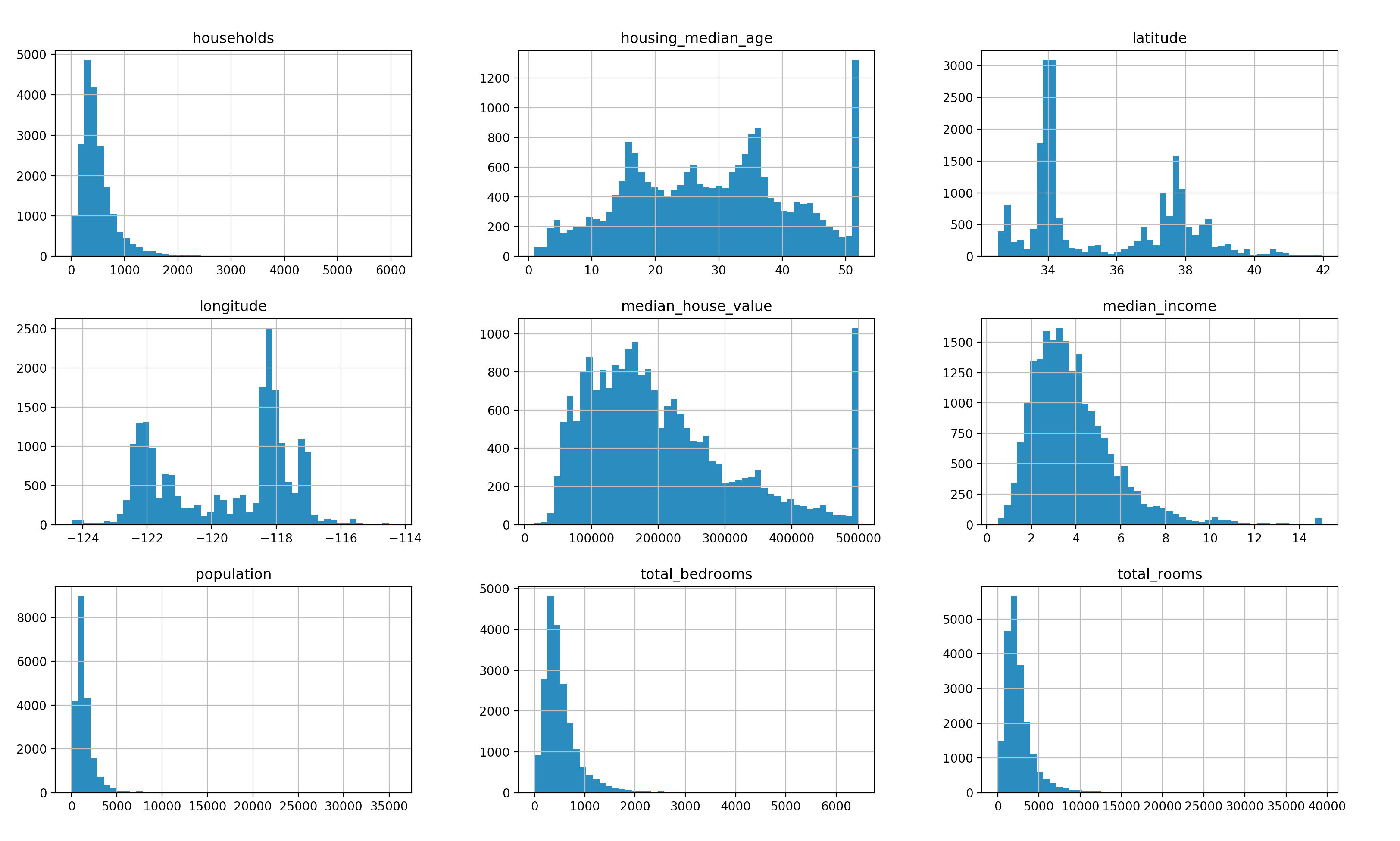
data = pd.read_csv("data/housing.csv")
data.hist(bins=50, figsize=(15, 12))
plt.show()

This code reads a CSV file, this file contains some information on the price. After reading through a histogram (hist) it shows up.

The contents of the CSV file can be found here: pandas_tutorial / the Data / housing.csv

Histogram results are as follows:

Conclusion

Although the title of this article is "Advanced chapter," We also discussed some of the more in-depth knowledge. But it is clear that for pandas is still very superficial things. Due to limited space, more content in the future, when we have the opportunity to come together to explore.

Readers may also be more in-depth study based on official documents online.

References and Recommended Reading

• pandas official website
• Python for Data Analysis

Original Address: https://paul.pub/advance-pandas/