NLP (xxi) the character of a real relation extraction

  Last year, I wrote an article using the relation extraction attempt to build knowledge map , trying to do with the relationship between open field now deep learning approaches extraction, but unfortunately, the current relationship in the open field extraction, has not ripe solutions and models. At that time the author of the article only as a first attempt, in actual use, the effect is limited.
  This article describes how to use the model to study the depth of character relation extraction. Characters relation extraction can be understood as the relationship extraction, which is an important step in building our knowledge map. The main idea of this paper is the relationship between the characters drawn relation extraction pipeline (pipeline) mode, because names can use ready-NER model extraction, this article only after solving the names extracted from the article, how to figure relation extraction.
  Depth learning model used in this paper is the text classification model, combined with BERT pre-training model, and achieved relatively good results.
  This project has been open source, Github address: https://github.com/percent4/people_relation_extract .
  FIG configuration item of the project as follows:

Dataset Introduction

  Before making attempts in this regard, we also have to face such a problem, that is the Chinese character of relations extracted corpus missing. Data is a prerequisite for the model, there is no data, all models of the question. Therefore, I had to spend a lot of time to collect data.
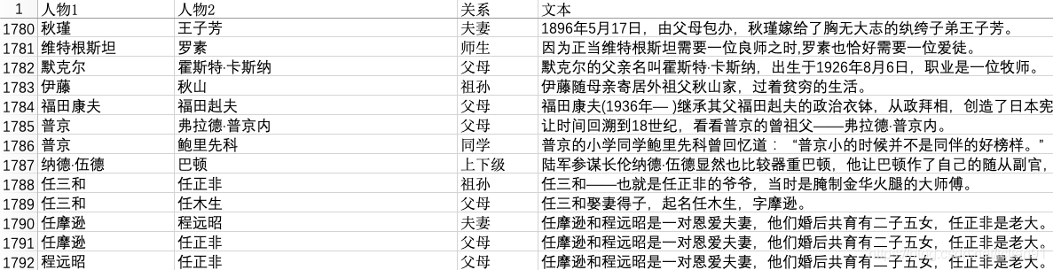
  I use a lot in your spare time, collected about 1800 relations sample persons, organized into Excel (file name 人物关系表.xlsx), the first few lines as follows:

the relationship between characters, a total of 14 categories, namely unknown, 夫妻, 父母, 兄弟姐妹, 上下级, 师生, 好友, 同学, 合作, 同人, 情侣, 祖孙, 同门, 亲戚, wherein the unknowncategory indicates the absence (no relationship between characters or other relation) of the person in relation to rest of the class 13, 同人the relationship between the two figures actually refers to the same person, as in the following example:

邵逸夫(1907年10月4日—2014年1月7日)，原名邵仁楞，生于浙江省宁波市镇海镇，祖籍浙江宁波。

In the above example, Shaw and Jen Shao flute is the same person. 亲戚Refers to the relationship in addition to 夫妻, 父母, 兄弟姐妹, 祖孙relatives outside, such as nephew, uncle and nephew relationship.
  For statistical relationship between the quantity of each category of data sets, we can use a script data/relation_bar_chart.py, complete Python code is as follows:

# -*- coding: utf-8 -*-
# 绘制人物关系频数统计条形图
import pandas as pd
import matplotlib.pyplot as plt

# 读取EXCEL数据
df = pd.read_excel('人物关系表.xlsx')
label_list = list(df['关系'].value_counts().index)
num_list= df['关系'].value_counts().tolist()

# Mac系统设置中文字体支持
plt.rcParams["font.family"] = 'Arial Unicode MS'

# 利用Matplotlib绘制条形图
x = range(len(num_list))
rects = plt.bar(left=x, height=num_list, width=0.6, color='blue', label="频数")
plt.ylim(0, 500) # y轴范围
plt.ylabel("数量")
plt.xticks([index + 0.1 for index in x], label_list)
plt.xticks(rotation=45) # x轴的标签旋转45度
plt.xlabel("人物关系")
plt.title("人物关系频数统计")
plt.legend()

# 条形图的文字说明
for rect in rects:
    height = rect.get_height()
    plt.text(rect.get_x() + rect.get_width() / 2, height+1, str(height), ha="center", va="bottom")

plt.show()

Results of operation as follows:

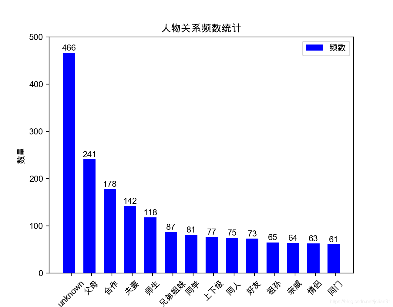
  unknowncategory most, there are 466, and the rest, such as 祖孙, 亲戚, 情侣, 同门and so more, only 60 pieces, because the lack of such data collection is not good relationships between the characters. Therefore, the corpus of the collection time-consuming, consumes a lot of energy.

Data preprocessing

  收集好数据后，我们需要对数据进行预处理，预处理主要分两步，一步是将人物关系和原文本整合在一起，第二步简单，将数据集划分为训练集和测试集，比例为8:2。
  我们对第一步进行详细说明，将人物关系和原文本整合在一起。一般我们给定原文本和该文本中的两个人物，比如：

邵逸夫(1907年10月4日—2014年1月7日)，原名邵仁楞，生于浙江省宁波市镇海镇，祖籍浙江宁波。

这句话中有两个人物：邵逸夫，邵仁楞， 这个容易在语料中找到。然后我们将原文本的这两个人物中的每个字符分别用'#'号代码，并通过'$'符号拼接在一起，形成的整合文本如下：

邵逸夫$邵仁楞$###(1907年10月4日—2014年1月7日)，原名###，生于浙江省宁波市镇海镇，祖籍浙江宁波。

处理成这种格式是为了方便文本分类模型进行调用。
  数据预处理的脚本为data/data_into_train_test.py，完整的Python代码如下：

# -*- coding: utf-8 -*-
import json
import pandas as pd
from pprint import pprint

df = pd.read_excel('人物关系表.xlsx')
relations = list(df['关系'].unique())
relations.remove('unknown')
relation_dict = {'unknown': 0}
relation_dict.update(dict(zip(relations, range(1, len(relations)+1))))

with open('rel_dict.json', 'w', encoding='utf-8') as h:
    h.write(json.dumps(relation_dict, ensure_ascii=False, indent=2))

pprint(df['关系'].value_counts())
df['rel'] = df['关系'].apply(lambda x: relation_dict[x])

texts = []
for per1, per2, text in zip(df['人物1'].tolist(), df['人物2'].tolist(), df['文本'].tolist()):
    text = '$'.join([per1, per2, text.replace(per1, len(per1)*'#').replace(per2, len(per2)*'#')])
    texts.append(text)

df['text'] = texts

train_df = df.sample(frac=0.8, random_state=1024)
test_df = df.drop(train_df.index)

with open('train.txt', 'w', encoding='utf-8') as f:
    for text, rel in zip(train_df['text'].tolist(), train_df['rel'].tolist()):
        f.write(str(rel)+' '+text+'\n')

with open('test.txt', 'w', encoding='utf-8') as g:
    for text, rel in zip(test_df['text'].tolist(), test_df['rel'].tolist()):
        g.write(str(rel)+' '+text+'\n')

运行完该脚本后，会在data目录下生成train.txt, test.txt和rel_dict.json，该json文件中保存的信息如下：

{
  "unknown": 0,
  "夫妻": 1,
  "父母": 2,
  "兄弟姐妹": 3,
  "上下级": 4,
  "师生": 5,
  "好友": 6,
  "同学": 7,
  "合作": 8,
  "同人": 9,
  "情侣": 10,
  "祖孙": 11,
  "同门": 12,
  "亲戚": 13
}

简单来说，是给每种关系一个id，转化成类别型变量。
  以train.txt为例，其前5行的内容如下：

4 方琳$李伟康$在生活中，###则把##看作小辈，常常替她解决难题。
3 佳子$久仁$12月，##和弟弟##参加了在东京举行的全国初中生演讲比赛。
2 钱慧安$钱禄新$###，生卒年不详，海上画家###之子。
0 吴继坤$邓新生$###还曾对媒体说：“我这个小小的投资商，经常得到###等领导的亲自关注和关照，我觉到受宠若惊。”
2 洪博培$乔恩·M·亨茨曼$###的父亲########是著名企业家、美国最大化学公司亨茨曼公司创始人。
10 夏乐$陈飞$两小无猜剧情简介:##和##是一对从小一起长大的青梅竹马。

在每一行中，空格之前的数字所对应的人物关系可以在rel_dict.json中找到。

模型训练

  在模型训练前，为了将数据的格式更好地适应模型，需要再对trian.txt和test.txt进行处理。处理脚本为load_data.py，完整的Python代码如下：

# -*- coding: utf-8 -*-
import pandas as pd


# 读取txt文件
def read_txt_file(file_path):
    with open(file_path, 'r', encoding='utf-8') as f:
        content = [_.strip() for _ in f.readlines()]

    labels, texts = [], []
    for line in content:
        parts = line.split()
        label, text = parts[0], ''.join(parts[1:])
        labels.append(label)
        texts.append(text)

    return labels, texts

# 获取训练数据和测试数据，格式为pandas的DataFrame
def get_train_test_pd():
    file_path = 'data/train.txt'
    labels, texts = read_txt_file(file_path)
    train_df = pd.DataFrame({'label': labels, 'text': texts})

    file_path = 'data/test.txt'
    labels, texts = read_txt_file(file_path)
    test_df = pd.DataFrame({'label': labels, 'text': texts})

    return train_df, test_df


if __name__ == '__main__':

    train_df, test_df = get_train_test_pd()
    print(train_df.head())
    print(test_df.head())

    train_df['text_len'] = train_df['text'].apply(lambda x: len(x))
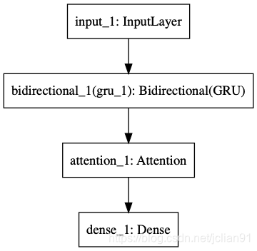
    print(train_df.describe())

  Model used in this project are: BERT + bi GRU + Attention + FC, which used to feature extraction BERT text, introduction to this part of the article is already in use BERT to achieve binary text NLP (XX) given in; attention is attention mechanisms layer, FC is a full connection layer, the structure of FIG model are as follows (using the derived Keras):

  model training script is model_train.pycomplete Python code as follows:

# -*- coding: utf-8 -*-
# 模型训练

import numpy as np
from load_data import get_train_test_pd
from keras.utils import to_categorical
from keras.models import Model
from keras.optimizers import Adam
from keras.layers import Input, Dense
from bert.extract_feature import BertVector

from att import Attention
from keras.layers import GRU, Bidirectional


# 读取文件并进行转换
train_df, test_df = get_train_test_pd()
bert_model = BertVector(pooling_strategy="NONE", max_seq_len=80)
print('begin encoding')
f = lambda text: bert_model.encode([text])["encodes"][0]

train_df['x'] = train_df['text'].apply(f)
test_df['x'] = test_df['text'].apply(f)
print('end encoding')

# 训练集和测试集
x_train = np.array([vec for vec in train_df['x']])
x_test = np.array([vec for vec in test_df['x']])
y_train = np.array([vec for vec in train_df['label']])
y_test = np.array([vec for vec in test_df['label']])
# print('x_train: ', x_train.shape)

# 将类型y值转化为ont-hot向量
num_classes = 14
y_train = to_categorical(y_train, num_classes)
y_test = to_categorical(y_test, num_classes)

# 模型结构：BERT + 双向GRU + Attention + FC
inputs = Input(shape=(80, 768,))
gru = Bidirectional(GRU(128, dropout=0.2, return_sequences=True))(inputs)
attention = Attention(32)(gru)
output = Dense(14, activation='softmax')(attention)
model = Model(inputs, output)

# 模型可视化
# from keras.utils import plot_model
# plot_model(model, to_file='model.png')

model.compile(loss='categorical_crossentropy',
              optimizer=Adam(),
              metrics=['accuracy'])

# 模型训练以及评估
model.fit(x_train, y_train, batch_size=8, epochs=30)
model.save('people_relation.h5')
print(model.evaluate(x_test, y_test))

The model of the training data set, the output results are as follows:

begin encoding
end encoding
Epoch 1/30
1433/1433 [==============================] - 15s 10ms/step - loss: 1.5558 - acc: 0.4962
**********(中间部分省略输出)**************
Epoch 30/30
1433/1433 [==============================] - 12s 8ms/step - loss: 0.0210 - acc: 0.9951
[1.1099, 0.7709]

The entire training process lasted ten minutes, trained 30 epoch, the ultimate loss on the test set is 1.1099, acc to 0.7709, the effect in a small amount of data is good.

Model predictions

  After the above model training, use the saved model file, the new data to predict. Model predictions for the script model_predict.py, complete Python code is as follows:

# -*- coding: utf-8 -*-
# 模型预测

import json
import numpy as np
from bert.extract_feature import BertVector
from keras.models import load_model
from att import Attention

# 加载模型
model = load_model('people_relation.h5', custom_objects={"Attention": Attention})

# 示例语句及预处理
text = '赵金闪#罗玉兄#在这里，赵金闪和罗玉兄夫妇已经生活了大半辈子。他们夫妇都是哈密市伊州区林业和草原局的护林员，扎根东天山脚下，守护着这片绿。'
per1, per2, doc = text.split('#')
text = '$'.join([per1, per2, doc.replace(per1, len(per1)*'#').replace(per2, len(per2)*'#')])
print(text)


# 利用BERT提取句子特征
bert_model = BertVector(pooling_strategy="NONE", max_seq_len=80)
vec = bert_model.encode([text])["encodes"][0]
x_train = np.array([vec])

# 模型预测并输出预测结果
predicted = model.predict(x_train)
y = np.argmax(predicted[0])

with open('data/rel_dict.json', 'r', encoding='utf-8') as f:
    rel_dict = json.load(f)

id_rel_dict = {v:k for k,v in rel_dict.items()}
print(id_rel_dict[y])

The results of the relationship between the characters is output 夫妻.
  Next, we predict better data, it outputs the result as follows:

原文: 润生#润叶#不过，他对润生的姐姐润叶倒怀有一种亲切的感情。
预测人物关系: 兄弟姐妹
原文: 孙玉厚#兰花#脑子里把前后村庄未嫁的女子一个个想过去，最后选定了双水村孙玉厚的大女子兰花。
预测人物关系: 父母
原文: 金波#田福堂#每天来回二十里路，与他一块上学的金波和大队书记田福堂的儿子润生都有自行车，只有他是两条腿走路。
预测人物关系: unknown
原文: 润生#田福堂#每天来回二十里路，与他一块上学的金波和大队书记田福堂的儿子润生都有自行车，只有他是两条腿走路。
预测人物关系: 父母
原文: 周山#李自成#周山原是李自成亲手提拔的将领，闯王对他十分信任，叫他担任中军。
预测人物关系: 上下级
原文: 高桂英#李自成#高桂英是李自成的结发妻子，今年才三十岁。
预测人物关系: 夫妻
原文: 罗斯福#特德#果然，此后罗斯福的政治旅程与长他24岁的特德叔叔如出一辙——纽约州议员、助理海军部长、纽约州州长以至美国总统。
预测人物关系: 亲戚
原文: 詹姆斯#克利夫兰#詹姆斯担任了该公司的经理，作为一名民主党人，他曾资助过克利夫兰的再度竞选，两人私交不错。
预测人物关系: 上下级（预测出错，应该是好友关系）
原文: 高剑父#关山月#高剑父是关山月在艺术道路上非常重要的导师，同时关山月也是最能够贯彻高剑父“折中中西”理念的得意门生。
预测人物关系: 师生
原文: 唐怡莹#唐石霞#唐怡莹，姓他他拉氏，名为他他拉·怡莹，又名唐石霞，隶属于满洲镶红旗。
预测人物关系: 同人

to sum up

  Depth learning model used in this paper is the text classification model, combined with BERT pre-training model, the amount of data in a small mark on the character of this relation extraction task has achieved good results. While the recognition accuracy of the model and use of lifting yet, I believe that the lifting point as follows:

• The need to increase the amount of data tagging, and now only about 1800 data, if the data volume up, and then the accuracy of the model range will also upgrade;
• Other models need to be more attempts;
• In the prediction, the prediction model is a long time, because the time-consuming extraction with BERT features, may be considered to shorten the time of the prediction model;
• Other issues are welcome to add.

  Thank you for reading ~

My micro-channel public number: Python's Wu (micro signal: easy_web_scrape), welcome attention ~