Optimal ratios calculated hedging
Cross-hedging refers to the underlying assets and quilt Paul inconsistencies assets in futures contracts, such as a company equipped with the SSE 180 Index ETF fund, but not the Shanghai Futures contracts 180 index on the market, the company can only choose the Shanghai and Shenzhen 300 index futures, Shanghai 50 CSI 500 index futures or index futures for hedging.
Optimal hedging ratio is also called the minimum variance hedging ratio, denoted h *, indicates how many futures contracts hedged asset price changes in a security unit needs to hedge. Construction of linear equations + [alpha] = H [Delta] S * × [Delta] F + [epsilon], where [Delta] S and [Delta] F respectively in the hedging period, changes apply security asset prices for futures and hedging price changes. Many times ΔS and ΔF with their daily return data instead. The linear regression calculation can be obtained H * = ρσ S / [sigma] F. = [Delta] S / [Delta] F, a process similar to find β coefficient of CAPM.
Assume that a fund company to configure the SSE 180 Index ETF fund, the company can only choose the Shanghai and Shenzhen 300 index futures contract IF1812, IH1812 SSE 50 Index futures contract or the CSI 500 Index futures contracts to hedge IC1812, listing the three contracts daily average is April 23, 2018, the last trading day is December 21, 2018, to select the most suitable contract according to the optimal hedging ratio.
step1: read SSE 180 Index ETF fund net and three futures contract settlement price data:
import numpy as np
import pandas as pd
data=pd.read_excel('C:/lenovo/Desktop/上证180ETF与期货合约.xlsx',index_col=0)
data.head()
Out[1]:
            上证180ETF  IF1812  IC1812  IH1812
交易日期
2018-04-23     3.218  3669.4  5524.0  2614.2
2018-04-24     3.278  3753.0  5681.8  2687.8
2018-04-25     3.261  3743.6  5677.4  2670.0
2018-04-26     3.216  3672.6  5598.8  2628.2
2018-04-27     3.217  3686.8  5612.6  2626.2
step2: the number generated each day for the return series:
SHre=np.log(data.iloc[:,0]/data.iloc[:,0].shift(1)).dropna()
IFre=np.log(data.iloc[:,1]/data.iloc[:,1].shift(1)).dropna()
ICre=np.log(data.iloc[:,2]/data.iloc[:,2].shift(1)).dropna()
IHre=np.log(data.iloc[:,3]/data.iloc[:,3].shift(1)).dropna()
step3: to three the number of futures contracts yield data as an argument, SSE 180 Index ETF logarithmic regression rate of return of the dependent variable respectively:
import statsmodels.api as sm
IF=sm.add_constant(IFre)
IC=sm.add_constant(ICre)
IH=sm.add_constant(IHre)
model1=sm.OLS(SHre,IF).fit()
model1.summary()
Out[3]:
<class 'statsmodels.iolib.summary.Summary'>
"""
                            OLS Regression Results
==============================================================================
Dep. Variable:               上证180ETF   R-squared:                     0.946
Model:                            OLS   Adj. R-squared:                  0.946
Method:                 Least Squares   F-statistic:                     2854.
Date:                Fri, 14 Feb 2020   Prob (F-statistic):          3.31e-105
Time:                        17:35:06   Log-Likelihood:                 715.08
No. Observations:                 165   AIC:                            -1426.
Df Residuals:                     163   BIC:                            -1420.
Df Model:                           1
Covariance Type:            nonrobust
==============================================================================
                 coef    std err          t      P>|t|      [0.025      0.975]
------------------------------------------------------------------------------
const          0.0002      0.000      0.628      0.531      -0.000       0.001
IF1812         0.8735      0.016     53.419      0.000       0.841       0.906
==============================================================================
Omnibus:                        1.256   Durbin-Watson:                   2.687
Prob(Omnibus):                  0.534   Jarque-Bera (JB):                0.866
Skew:                           0.114   Prob(JB):                        0.648
Kurtosis:                       3.271   Cond. No.                         65.8
==============================================================================
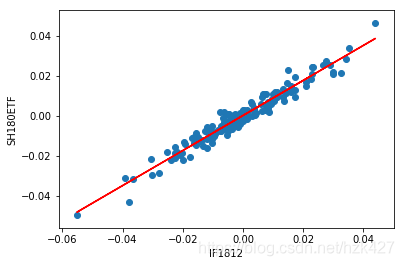
Similarly available other two futures linear regression model results, the coefficient of determination R & lt 2 were 0.72 and 0.929, most hedge ratio of 0.922 and 0.6657, respectively. In terms of R & lt 2 highest as the optimum model is selected, the security contract IF1812 contract as the most appropriate condom, R & lt 2 reached 0.946, most hedge ratio of .8735. Paint can look at fitting effect:
import matplotlib.pyplot as plt
plt.plot(IFre,model1.params[0]+model1.params[1]*IFre,'r-')
plt.scatter(IFre,SHre,marker='o')
plt.xlabel('IF1812')
plt.ylabel('SH180ETF')
Optimal number of futures hedging contracts
Then calculate how much the number of futures contracts hedgers need for hedging operations. Suppose Q S indicates the number of assets insured quilt, Q F. Represents the size of a futures contract, N * represents most futures contracts for hedging parts, then there × Q * N F. × [Delta] F = Q S × [Delta] S, substituting h * = ΔS / ΔF * = H * have Q N S / Q F. .
Connected cases, assuming that the fund company bought in December 28, 2018 in accordance with the closing net 2.768 yuan SSE 180 Index ETF billion, while the CSI 300 futures IF1901 contracts with short positions (daily settlement price of 3003.6 yuan) to set Paul, assuming optimal hedge ratios constant, seeking the best futures of contracts:
def n(h,qs,qf):
	return h*qs/qf
n(model1.params[1],100000000,3003.6*300)
Out[6]: 96.9344687900856
So IF1901 contract to sell 97 copies.
Dynamic Break combined hedging
Connected cases, it is assumed that after completion of hedging, with changes in NAV and futures contract prices, the overall effect of hedging portfolio also changed, calculate the three trading portfolio hedging profit and loss information in the following table:
| date | January 11, 2019 | January 14, 2019 | January 15, 2019 |
|---|---|---|---|
| NAV (yuan) | 2.836 | 2.815 | 2.867 |
| Futures contract settlement price | 3095.0 | 3069.4 | 3126.2 |
net0=2.768;N=97;F0=3003.6;Q=100000000
net=pd.Series([2.836,2.815,2.867])
F=pd.Series([3095.0,3069.4,3126.2])
for i in range(3):
	r=Q*((net[i]/net0)-1)-300*N*(F[i]-F0)#这时用一般收益率公式更合理
	print('第{}个交易日套保组合的累积盈亏为{:.2f}'.format(i+1,r))

第1个交易日套保组合的累积盈亏为-203092.60
第2个交易日套保组合的累积盈亏为-216803.12
第3个交易日套保组合的累积盈亏为8929.60
Visible hedging calculate the optimal ratio not once, in order to obtain the best effect of hedging, consider creating a dynamic model of such hedging DCC-GARCH, Copula like.
