We introduce in the chapter notes the theoretical knowledge Perceptron, discusses the origin of perception machine works, solving strategies, convergence. In this note, we have to write your own code, Perceptron algorithm to solve practical problems.
Start with a simple question to start, with the Perceptron algorithm to solve classification OR logic.
import numpy as np
import matplotlib.pyplot as plt

x = [0,0,1,1]
y = [0,1,0,1]

plt.scatter(x[0],y[0], color="red",label="negative")
plt.scatter(x[1:],y[1:], color="green",label="positive")

plt.legend(loc="best")
plt.show()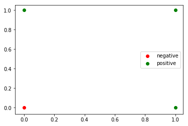
Let's define a function used to determine whether a sample point is correctly classified. Since the sample points in this example is two-dimensional, and therefore also the weight vector corresponding two-dimensional, can be defined as \ (W = (W_1, w_2) \) , the list may be used in Python be expressed, for example w = [0, 0], to the sample hyperplane distance is natural w[0] * x[0] + w[1] * x[1] +b. Here are the complete function.
def decide(data,label,w,b):
    result = w[0] * data[0] + w[1] * data[1] - b
    print("result = ",result)
    if np.sign(result) * label <= 0:
        w[0] += 1 * (label - result) * data[0]
        w[1] += 1 * (label - result) * data[1]
        b += 1 * (label - result)*(-1)
    return w,b
After writing the core function, we need to write a dispatch function that provides functionality to traverse each sample point.
def run(data, label):
    w,b = [0,0],0
    for epoch in range(10):
        for item in zip(data, label):
            dataset,labelset = item[0],item[1]
            w,b = decide(dataset, labelset, w, b)
            print("dataset = ",dataset, ",", "w = ",w,",","b = ",b)
    print(w,b)
data = [(0,0),(0,1),(1,0),(1,1)]
label = [0,1,1,1]run(data,label)result = 0
dataset = (0, 0) , w = [0, 0] , b = 0
result = 0
dataset = (0, 1) , w = [0, 1] , b = -1
result = 1
dataset = (1, 0) , w = [0, 1] , b = -1
result = 2
dataset = (1, 1) , w = [0, 1] , b = -1
result = 1
dataset = (0, 0) , w = [0, 1] , b = 0
result = 1
dataset = (0, 1) , w = [0, 1] , b = 0
result = 0
dataset = (1, 0) , w = [1, 1] , b = -1
result = 3
dataset = (1, 1) , w = [1, 1] , b = -1
result = 1
dataset = (0, 0) , w = [1, 1] , b = 0
result = 1
dataset = (0, 1) , w = [1, 1] , b = 0
result = 1
后面的迭代这里省略不贴,参数稳定下来,算法已经收敛Let's look at a data set from the UCI: PIMA diabetes dataset, examples from Chapter 3, "the perspective of the machine learning algorithm"
import os
import pylab as pl
import numpy as np
import pandas as pdos.chdir(r"DataSets\pima-indians-diabetes-database")pima = np.loadtxt("pima.txt", delimiter=",", skiprows=1)pima.shape(768, 9)indices0 = np.where(pima[:,8]==0)
indices1 = np.where(pima[:,8]==1)pl.ion()
pl.plot(pima[indices0,0],pima[indices0,1],"go")
pl.plot(pima[indices1,0],pima[indices1,1],"rx")
pl.show()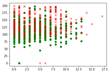
Data preprocessing
1. The age of discrete
pima[np.where(pima[:,7]<=30),7] = 1
pima[np.where((pima[:,7]>30) & (pima[:,7]<=40)),7] = 2
pima[np.where((pima[:,7]>40) & (pima[:,7]<=50)),7] = 3
pima[np.where((pima[:,7]>50) & (pima[:,7]<=60)),7] = 4
pima[np.where(pima[:,7]>60),7] = 5
2. The unified number of pregnancies of women with more than 8 times 8 times instead of
pima[np.where(pima[:,0]>8),0] = 83. The data normalized
pima[:,:8] = pima[:,:8]-pima[:,:8].mean(axis=0)
pima[:,:8] = pima[:,:8]/pima[:,:8].var(axis=0)
4. segmentation training and testing sets
trainin = pima[::2,:8]
testin = pima[1::2,:8]
traintgt = pima[::2,8:9]
testtgt = pima[1::2,8:9]
Definition Model
class Perceptron:
    def __init__(self, inputs, targets):
        # 设置网络规模
        # 记录输入向量的维度,神经元的维度要和它相等
        if np.ndim(inputs) > 1:
            self.nIn = np.shape(inputs)[1]
        else:
            self.nIn = 1

        # 记录目标向量的维度,神经元的个数要和它相等
        if np.ndim(targets) > 1:
            self.nOut = np.shape(targets)[1]
        else:
            self.nOut = 1

        # 记录输入向量的样本个数
        self.nData = np.shape(inputs)[0]

        # 初始化网络,这里加1是为了包含偏置项
        self.weights = np.random.rand(self.nIn + 1, self.nOut) * 0.1 - 0.05

    def train(self, inputs, targets, eta, epoch):
        """训练环节"""
        # 和前面处理偏置项同步地,这里对输入样本加一项-1,与W0相匹配
        inputs = np.concatenate((inputs, -np.ones((self.nData,1))),axis=1)

        for n in range(epoch):
            self.activations = self.forward(inputs)
            self.weights -= eta * np.dot(np.transpose(inputs), self.activations - targets)
        return self.weights

    def forward(self, inputs):
        """神经网路前向传播环节"""
        # 计算
        activations = np.dot(inputs, self.weights)
        # 判断是否激活
        return np.where(activations>0, 1, 0)

    def confusion_matrix(self, inputs, targets):
        # 计算混淆矩阵
        inputs = np.concatenate((inputs, -np.ones((self.nData,1))),axis=1)
        outputs = np.dot(inputs, self.weights)
        nClasses = np.shape(targets)[1]

        if nClasses == 1:
            nClasses = 2
            outputs = np.where(outputs<0, 1, 0)
        else:
            outputs = np.argmax(outputs, 1)
            targets = np.argmax(targets, 1)

        cm = np.zeros((nClasses, nClasses))
        for i in range(nClasses):
            for j in range(nClasses):
                cm[i,j] = np.sum(np.where(outputs==i, 1,0) * np.where(targets==j, 1, 0))
        print(cm)
        print(np.trace(cm)/np.sum(cm))
print("Output after preprocessing of data")
p = Perceptron(trainin,traintgt)
p.train(trainin,traintgt,0.15,10000)
p.confusion_matrix(testin,testtgt)
Output after preprocessing of data
[[ 69.  86.]
 [182.  47.]]
0.3020833333333333
In this case the use of the results obtained by Perceptron training relatively poor, here only as an example to show the algorithm.
Perceptron last look at an example of digital handwriting recognition algorithm MNIST use. Kernel code that draws on Kaggle.
step 1: introducing the desired first packet, and set the path where the data
import numpy as np
import pandas as pd
import matplotlib.pyplot as plt
train = pd.read_csv(r"DataSets\Digit_Recognizer\train.csv", engine="python")
test = pd.read_csv(r"DataSets\Digit_Recognizer\test.csv", engine="python")print("Training set has {0[0]} rows and {0[1]} columns".format(train.shape))
print("Test set has {0[0]} rows and {0[1]} columns".format(test.shape))Training set has 42000 rows and 785 columns
Test set has 28000 rows and 784 columnsstep 2: Data Preprocessing
Created
label, its size is (42000 1)Create
training set, size is (42000, 784)Create
weights, size is(10,784), it may be a bit difficult to understand. We know that the weight vector is a description of neurons, 784 is the dimension that represents a 784-dimensional input sample corresponding neurons and it also has a 784-dimensional docking. At the same time, remember that a neuron can only output a output, and digital identification problem, we look forward to a sample of the input data, can return to 10 digits, then the probability that the sample is judged according to what number of maximum likelihood. So, we need 10 neurons, which is the(10,784)origin.
trainlabels = train.label
trainlabels.shape(42000,)traindata = np.asmatrix(train.loc[:,"pixel0":])
traindata.shape(42000, 784)weights = np.zeros((10,784))
weights.shape
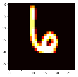
(10, 784)Here you can look at a sample, look feel. Note that the original data is compressed into 784-dimensional array, we need to change it back to the picture 28 * 28
# 从矩阵中随便取一行
samplerow = traindata[123:124]
# 重新变成28*28
samplerow = np.reshape(samplerow, (28,28))
plt.imshow(samplerow, cmap="hot")
step 3: Training
Here we cycle several times on the training data set, and then focus on error rate curve
# 先创建一个列表,用来记录每一轮训练的错误率
errors = []
epoch = 20

for epoch in range(epoch):
    err = 0
    # 对每一个样本(亦矩阵中的每一行)
    for i, data in enumerate(traindata):
        # 创建一个列表,用来记录每个神经元输出的值
        output = []
        # 对每个神经元都做点乘操作,并记录下输出值
        for w in weights:
            output.append(np.dot(data, w))
        # 这里简单的取输出值最大者为最有可能的
        guess = np.argmax(output)
        # 实际的值为标签列表中对应项
        actual = trainlabels[i]

        # 如果估计值和实际值不同,则分类错误,需要更新权重向量
        if guess != actual:
            weights[guess] = weights[guess] - data
            weights[actual] = weights[actual] + data
            err += 1
    # 计算迭代完42000个样本之后,错误率 = 错误次数/样本个数
    errors.append(err/42000)
x = list(range(20))
plt.plot(x, errors)
[<matplotlib.lines.Line2D at 0x5955c50>]
As can be seen from the figure, up to 15 iterations, the error rate has been a rising trend, and began to live a fit.
Perceptron is a very simple algorithm, that it is difficult to use Perceptron algorithm in a real scene. Three examples cited here, it is intended to write code that implements the algorithm hands, look feel. More experienced readers must be wondering: Why not use Scikit-Learn this package, this part is actually the author had other plans, we intend to combine algorithm written Scikit-Learn interpretation of source notes. Of course, limited to the individual level, it may not be able to resolve the essence, but rather as it managed to. Part II will write Multi-Layer-Perceptron algorithm theory, where we can easily see, even a simple machine perception, just add a hidden layer, it can significantly improve the classification ability. In addition, you will find time to write a perception interpretation of the source machine Sklearn article. Have any questions, welcome to discuss the message.