We know that the earlier classification model - Perceptron (1957) is a second-class classification of linear classification model, but also was the basis of neural networks and support vector machine. SVM (Support vector machines) is a second-class earliest classification model, through evolution, it has now become not only handle multiple linear and nonlinear problems, but also to deal with the problem return. Before swept depth study should be regarded as the best classification algorithm . But there are still a lot of SVM applications, especially on a small sample set.
First, the table of contents
1. List
2, Perceptron
3, the hard interval SVM
4, soft margin support vector machine
5, hinge loss function
Second, Perceptron ( foreplay )
Perceptron model is a binary linear classifier, can handle only linearly separable problems, perceptual model machine is to try to find a hyperplane to separate data set, this hyperplane is a straight line in two-dimensional space, three-dimensional space is a plane. Perceptron classification model are as follows:


Machine is perceived hyperplane wx + b = 0.
The above functions are integrated into the segment y * (wx + b)> 0, the equation is satisfied, i.e., sample points correctly classified point, i.e. the point does not satisfy the classification error, our goal is to find a set of parameters such w , b separated so that the training set positive and negative points for point class.

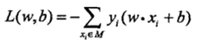
Next, we define a function loss (loss function is a measure of the degree of error and loss of function), we can define the number of misclassified samples as a function of the loss, but this is not the loss function parameters w, b of continuously differentiable function, it is not easy to optimize. We know that for misclassified points
There -y (wx + b)> 0 , we let all of misclassification point to hyperplane distance and minimum (note : the perceived loss function machine for misclassification point, rather than the entire set of training only ):
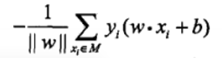
Where M is a sample set of misclassifications, when w, b multiples increase and does not change our hyperplane, the value of || W || accordingly increased, and thus make || W || = 1 does not affect our results. The final Perceptron loss function as follows:
Third, the hard interval and SVM
Function interval:
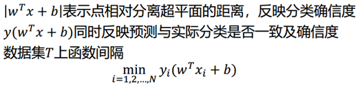
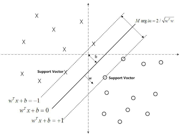
In the above formula do not function properly spaced reaction point hyperplane distance , we also mentioned the perceptron model, when the molecule is proportional to the growth, the denominator is doubled. To measure unity, we need to add constraints normal vector w, so that we get the geometric spacing gamma], the following equation defines the distance of the nearest point hyperplane, i.e. the support point (which is the name of the source of support vector machines), defined as:

The following claim is the maximum interval hyperplane: separate if all samples only can be a hyperplane, further and hyperplane maintain a certain function of the distance (at a function distance 1), then this hyperplane than perceptron Classification optimal hyperplane. Can prove that such a super-plane only. And two hyperplanes corresponding vector remains parallel hyperplanes certain function of the distance, which we define as the support vector, as shown in phantom in FIG.
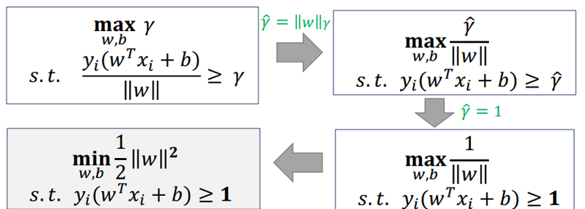
Description: γ (hat) is a function of the separation, and the value of the interval will function as w, b into the fold change varies, and not affect the final result, and therefore make the gamma] (hat) = 1, then our ultimate problem can be stated as:

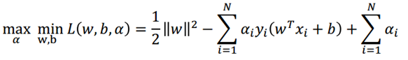
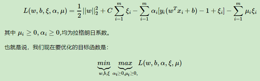
The above problems 1/2 || w || 2 is a convex function, while the inequality constraint is an affine function, so this is a convex quadratic programming problem, according to the theory of convex optimization, we can use a Lagrangian our constraint problem into unconstrained problem to solve, our optimization function can be expressed as:

: The following is the process of solving the
problem according to the duality [can be converted to the original problem of Lagrange dual problem (as long as there is the dual problem, dual problem to resolve is the best of the best to resolve the original problem, dual problem than the original general easier to solve) Minimax problem:

First of w, b seeking min Problems derivative can be obtained value w, b of:

The solution obtained is substituted into the Lagrangian function can be obtained following optimization function (to be substituted into the originally great problem of seeking converted into α min Problems):
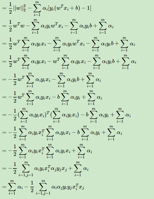
Substitution process described above, whereby the following results were obtained:

Thus we obtained only required value of α can be determined our w, the value of b (α is commonly used algorithm for SMO algorithm can refer https://www.cnblogs.com/pinard/p/6111471.html) [alpha] finally obtained assumed a value of α *, the w, b can be expressed as:

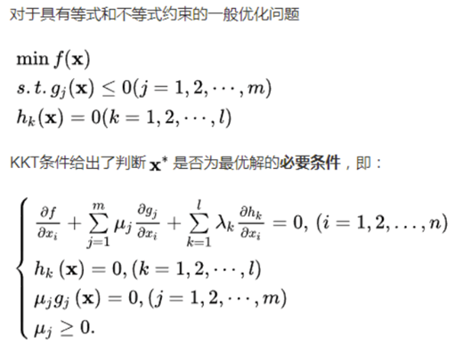
KTT introduced conditions (with the proviso that the above Lagrangian KTT prerequisite seeking the optimal solution):
As it can be seen from KTT conditions , when yi (w * xi + b * ) - when 1> 0, αi * = 0 ; if αi *> time 0, yi (w * xi + b *) - 1 = 0;
Combination of the above w, b expression can lead SVM second highlight: w, b parameter is only satisfying yi (w * xi + b * ) - 1 = 0 samples, whereas the samples from the maximum point is interval hyperplane nearest point, we will call these points support vector . So many times a good support vector classification in small sample sets can be represented, it is precisely because of this reason. (Also note: the number of vector α is set equal to the number of training and, for large training set, will cause an increase in the number of parameters required, so SVM will learn to process large training set than other common machine algorithm slower)
Fourth, the soft margin support vector machine
Linearly separable nonlinear SVM to learn the data set is no way to use because sometimes not linearly separable linear data set is more than a small number of which outliers, since these lead to outlier data set can not be linearly points, then how can deal with these outliers can still use the data set linearly separable thought it? Description Soft maximize spaced linear SVM here. Figure shows the importance of soft under two intervals:


Shown, usually some noise, or above the training set, there will be some anomalies FIG point, which can lead to abnormal points linearly inseparable training set, but then these outliers removed, the remaining sample is linearly separable, while the upper hard maximize the mentioned intervals can not deal with the problem of linearly inseparable, means linearly inseparable function of some sample point interval is not greater than or equal to satisfy constraints 1. Therefore, we introduce a per sample (xi, yi) slack variables ξi , then we constraint becomes:
The objective function:

[Simple comparison]

[Problem-solving]
Lagrangian function:
First, we find an optimization function for w, b, ξ is the minimum value, the partial derivative can be obtained by:

Into the formula:

So simplifies to:
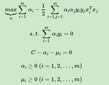
For C-αi-μi = 0, αi≥0, μi≥0 these three equations, we can eliminate μi, leaving only αi, that is to say 0≤αi≤C. The objective function while the variable number, find the minimum value, again simplifying :
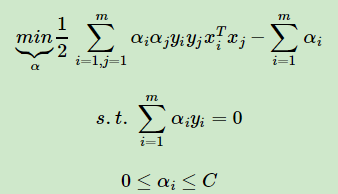
This is the form of linear optimization goal of maximizing the time interval can be divided into soft SVM's, and maximizing the linear SVM can be divided into hard interval above comparison, we just have one more constraint 0≤αi≤C . We can find the corresponding still when the vector α formula minimization algorithm can be determined by SMO w a and b.
When maximize soft interval, slightly more complicated, because we have introduced slack variables ξi for each sample (xi, yi). From the figure we have to study the situation of support vectors is maximized soft interval, the i-th point to the corresponding categories of support for distance vector. According to the complementary of the dual maximized soft interval KKT conditions:


Fifth, the hinge loss function
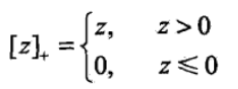
The introduction to the first: hinge loss function, also known as hinge loss function, which was expressed as follows:
Linear support vector machine there is another explanation follows:

Where L (y (w ∙ x + b)) = [1-yi (w ∙ x + b)] + loss function is called hinge (hinge loss function).
The first of the above-described loss function may be understood that when the sample interval is greater than 1 and the classification accuracy, i.e. yi (wxi + b) ≥ 1, the loss is 0; and when yi (wxi + b) <1, loss 1 - yi (wxi + b) , note that even if the sample where the correct classification, but also counted interval is less than a loss, which is the severity of the support vector machine . The figure is relatively hinge loss function and some other loss function:

Green line, if the points are correctly classified, and the function of the separation is greater than 1, the loss is 0, or loss 1-y (w ∙ x + b);
Black line: 0-1 for the loss function, if the correct classification, the loss is 0, 1 misclassification costs,
Purple line: 0-1 loss function is not visible guide. For perceptron model, perceptual loss function machine is [-yi (w ∙ x + b)] +, so that when the sample is correctly classified, the loss is 0, when the misclassification loss -yi (w ∙ x + b );
For logistic regression or the like and the maximum entropy model corresponding to the number of losses, loss of function is the log [1 + exp (-y (w ∙ x + b))].