Spatial Transformer Networks
Brief introduction
This paper proposes a structure capable of learning feature affine transformation, and the structure does not require additional supervision to other information networks themselves will be able to learn useful in predicting the results of an affine transformation. Because the spatial characteristics CNN translation invariance to some extent been destroyed pooling and other operations, so you want to be able to respond to network or other object after object affine transformation better representation of translation, we need to design a structure learning this transformation, so that the role of this transformed feature can be able to express good job.
Network architecture

U represents the figure above the input feature map, the branch learned by transform spatial transformer, and then mapped to the output difference or other feature by sampler, feature so that the output will have a more robust representation.
spatial transform structure consists of three parts, described in detail below.
Affine transformation
Affine transformation into pan, zoom, flip, rotate, and converting these types of crop, wherein the two dimensional transform matrix can be represented by:
\ [\ left (\} the begin Matrix {X '\\ Y' \ {End Matrix } \ right) = \ left [ \ begin {matrix} \ theta_1 & \ theta_2 & \ theta_3 \\ \ theta_4 & \ theta_5 & \ theta_6 \\ \ end {matrix} \ right] \ left (\ begin {matrix} x \\ y \\ 1 \ end {matrix
} \ right) \] wherein the corresponding theta take different values corresponding to different transform. So the students learn this network transformation, help feature to get a more effective representation.
Localisation Network
The portion localisation net portion corresponding to the figure above, the purpose is to study the parameters theta in the above formula, that is to say, the structure of this part may be directly connected to a full or 6 theta using conv structure as long as can be mapped to 6 theta on it. This is the easy part.
Parameterised Sampling Grid
This portion corresponds to a portion of FIG Grid Generator, the role of this part is mapped to the output image to establish the position of the input image position, i.e. corresponding to the affine transformation we mentioned above, we can learn from the above structure in this theta parameter to be put through affine transformation of the input matrix, when attention transformed transform each channel should be the same. Formula is expressed as:
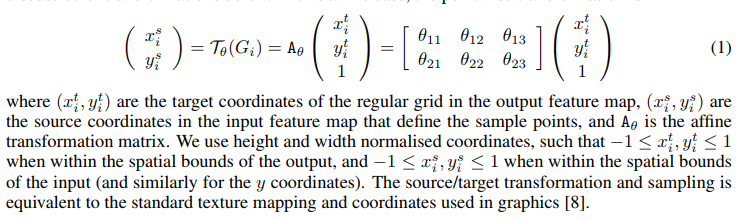
We can define the network by limiting theta values learning only a transformation, that is only part of learning theta parameters.
Differentiable Image Sampling
The above affine transformation only defines the location of mapping transform to transform the former, in fact, this mapping is not complete, which means that some point is no value, If you give value, then use the interpolation method. The paper mentions the nearest neighbor interpolation and bilinear interpolation two kinds of interpolation methods.
For the nearest neighbor interpolation such a definition is given:
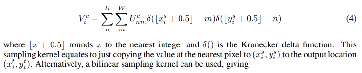
Thus for the i-th value of the output of the feature, the position of the corresponding input feature depends on m and n, defined by the known krnoecker delta function, if and only if the output is 0 to 1. Therefore, the argument is only made in the above formula m the x-direction from the point corresponding to the point nearest integer value as well as the nearest point on the integer n to obtain the y direction, which corresponds to a value for the values in both directions of the nearest point.
For bilinear interpolation gives this definition:
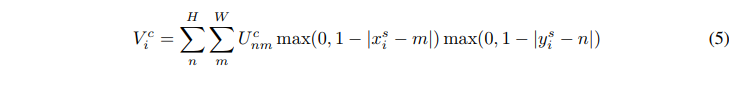
Can be known from the above equation, only the value only when the value of m and n is an integer within a corresponding point on the xy direction distance, and the distance to the nearest integer corresponding point is four points, such as (0.5, 0.5) from its four nearest points are (0,0), (0,1), (1,1), (1,0), it would be behind the two distance weight value, a value of four front U an integer value of one point of the points, so the equation can be interpreted as a distance weight, rounded to the nearest point weighted summation of four values.
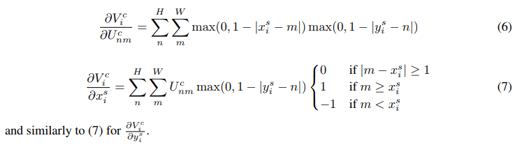
Back Propagation
Corresponds to the function defined above, the authors demonstrated that the input to the output may be made counter-propagating to bilinear interpolation as an example: