The area under the ROC curve R language - Evaluation Discrimination Logic Regression

Original link: http://tecdat.cn/?p=6310

 

 

Before discussing the ROC curve, let us consider the difference between calibration and discrimination in the context of logistic regression. 

 

Good calibration is not enough

 

For the model covariates given value, the probability that we can get predictable. If you look at the risks and risk prediction (probability) matches, the model is said to have been well calibrated. That is, if we want to allocate a large number of observations of a set of values, the proportion of these observations should be close to 20%. If the observed proportion is 80%, we might agree that the poor performance of the model - which underestimated the risks of these observations. Should we be satisfied with the use of the model, as long as it is well-calibrated? Unfortunately. To understand why, we assume a model fitted to our results but there is no covariates, i.e. model: log probability, so that the predicted value of the same ratio observed with the data set. The (quite useless) model to predict the probability of each observation allocated the same. It has a good calibration - the next sample, the observed ratio will be close to our estimate of the probability. However, this model is not really useful, because it does not distinguish between high-risk and low-risk observation observation. This is similar to the weatherman, who every day say the chance of rain tomorrow is 10%. This prediction may have been well calibrated, but it does not tell people whether the possibility of a more or less rain, so not really a useful predictor!

 

ROC curve plotted in R 
 

set.seed（63126）
n < -  1000
x < -  rnorm（n）
pr < -  exp（x）/（1 + exp（x））
y < -  1 *（runif（n）<pr）
mod < -  glm（y~x，family =“binomial”）

Next, the probability of vector fitting we extract objects from the model fitting in:

predpr < -  predict（mod，type = c（“response”））

We are now loaded pROC package, and generates a roc roc object using the function. The basic syntax is specified type regression equation, the left side is the response y, the probability of fitting the right is an object comprising:

 roccurve < -  roc（y~preppr）

You can then use to draw objects roc

 ​

This gives us the ROC plot (see previous figure). Note here because our logistic regression model contains only a covariate, if we use roc (y ~ x), ROC curves look identical, i.e., we do not need fitted logistic regression models. This is because only a covariate, the only fitting probability is a monotonic function of covariates. However, in general (i.e., more than one model covariate), is not the case.

We said before a good model has the ability to identify, ROC curve will be close to the upper left corner. To this point, we will re-examination by simulating analog data, the log odds ratios from 1 to 5:

set.seed（63126）
n < -  1000
x < -  rnorm（n）
pr < -  exp（5 * x）/（1 + exp（5 * x））
y < -  1 *（runif（n）<pr）
mod < -  glm（y~x，family =“binomial”）

predpr < -  predict（mod，type = c（“response”））

roccurve < -  roc（y~preppr）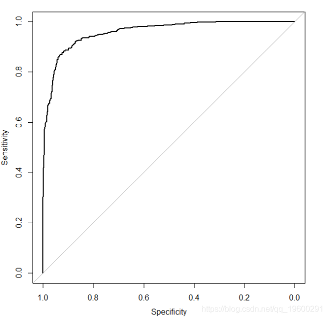

​

 

 Now let's run the simulation again, but in fact nothing to do with the variable x y. To this end, we only need to modify the line to generate the probability vector pr

pr < -  exp（0 * x）/（1 + exp（0 * x））

It gives the following ROC curve

​

 

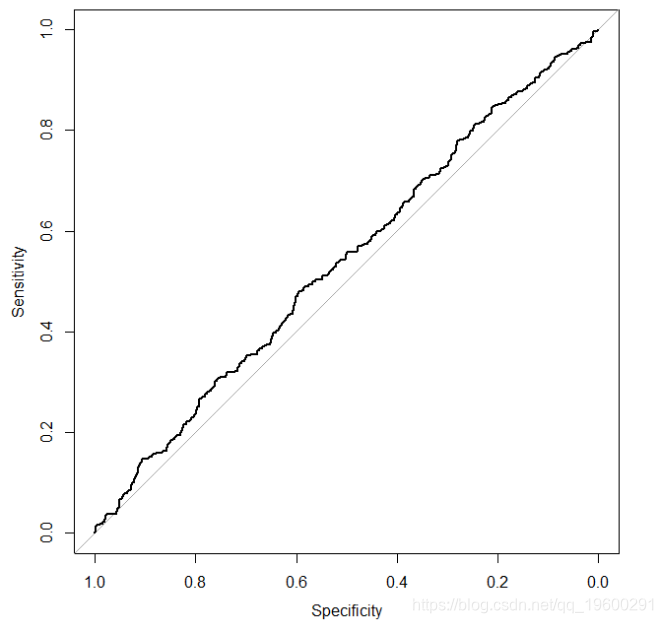
ROC curve, regardless of the predictors which results

 

The area under the ROC curve

Summarizes the ability of the model to identify a popular way is to report the area under the ROC curve. We have seen that the model has the ability to identify with a figure closer to the upper left corner of the ROC curve, and no model has the ability to identify close to 45-degree line of the ROC curve. Thus, from an area under the curve (corresponding to perfect discrimination) to 0.5 (corresponding to no ability to distinguish the model). The area under the ROC curve is also sometimes called c statistic (c represent consistency).

 

Thank you for reading this article, you have any questions please leave a comment below!

 

 

Big Data tribe - Chinese professional third-party data service providers to provide customized one-stop data mining and statistical analysis consultancy services

Statistical analysis and data mining consulting services: y0.cn/teradat (Consulting Services, please contact the official website customer service )

QQ：3025393450

 

[Service] Scene  

Research projects; 

 

Companies outsourcing; online and offline one training; data collection; academic research; report writing; market research.

[Tribe] big data to provide customized one-stop data mining and statistical analysis consultancy services

Share the latest information about big data, data analysis, study a little every day, so we do have the attitude of people together data

Micro-channel customer service number: lico_9e

QQ exchange group: 186 388 004 

Welcome to elective our R language data analysis will be mining will know the course!

 

Welcome attention to micro-channel public number for more information about data dry!