Table of Contents of Series Articles
代码:https://jumpat.github.io/SAGA.
论文:https://jumpat.github.io/SAGA/SAGA_paper.pdf
来源:上海交大和华为研究院
Article directory
Summary
Interactive 3D segmentation technology is of great significance in 3D scene understanding and manipulation and is a task worthy of attention. However, existing methods face challenges in achieving fine-grained, multi-granular segmentation or contend with substantial computational overhead, inhibiting real-time interaction. In this paper, we introduce Segmented Arbitrary 3D Gassin (SAGA), a new 3D interactive segmentation method that seamlessly combines 2D segmentation models with 3D Gaussian Splatting (3DGS). SAGA effectively embeds the multi-granularity 2D segmentation results generated by the segmentation model into 3D Gaussian point features through well-designed contrast training . Experimental evaluation demonstrates competitive performance. In addition, SAGA can complete 3D segmentation in milliseconds, also implements multi-granularity segmentation, and adapts to various cues, including points, graffiti, and 2D masks.
I. Introduction
Three-dimensional interactive segmentation has attracted widespread attention from researchers due to its potential applications in fields such as scene manipulation, automatic labeling, and virtual reality. Previous methods [13, 25, 46, 47 Decomposing nerf, Neural feature fusion fields, etc.] mainly promote two-dimensional visual features into three-dimensional space through training feature fields to simulate self-supervised visual models [4, 39] Extracted multi-view 2D features. Three-dimensional feature similarity is then used to measure whether two points belong to the same object. This approach is fast due to its simple segmentation pipeline, but at the cost of coarse segmentation granularity due to the lack of mechanisms to parse the information embedded in the features (e.g., segmentation decoders). In contrast, another paradigm [5: Segment anything in 3d with nerfs] improves the 2D segmentation basic model to a 3D model by directly projecting multi-view fine-grained 2D segmentation results onto a 3D mask grid. . Although this method can produce accurate segmentation results, its large time overhead limits interactivity due to the need to execute the underlying model and rendering multiple times.
The above discussion reveals the dilemma of existing paradigms in achieving efficiency and accuracy, and points out two factors that limit the performance of existing paradigms. First, the implicit radiation fields employed by previous methods [5, 13] hinder effective segmentation : three-dimensional space must be traversed to retrieve a three-dimensional object. Secondly, by utilizing a two-dimensional segmentation decoder, the segmentation quality is high but the efficiency is low.
Three-dimensional Gaussian Splatting (3DGS) is capable of high-quality and real-time rendering : it uses a set of three-dimensional color Gaussian distributions to represent a three-dimensional scene. The average of these Gaussian distributions represents their position in three-dimensional space, so 3DGS can be viewed as a point cloud that helps bypass the extensive processing of huge, often empty three-dimensional spaces and provides rich Explicit three-dimensional priors. With this point cloud-like structure, 3DGS not only achieves efficient rendering but also becomes an ideal candidate for segmentation tasks.
On the basis of 3DGS, we proposed Segment Any 3D GAussians (SAGA) : extracting the fine-grained segmentation capabilities of the 2D segmentation model (i.e. SAM) into a 3D Gaussian model, focusing on upgrading 2D visual features to 3D, and achieving Fine-grained 3D segmentation . Furthermore, it avoids multiple inferences of the 2D segmentation model. Distillation is implemented using SAM to automatically extract masks and train three-dimensional features of Gaussian distribution. During inference, an input hint is used to generate a set of queries, which are then used to retrieve the desired Gaussian through efficient feature matching . The method enables fine-grained 3D segmentation in milliseconds and supports a variety of cues, including points, doodles, and masks.
2. Related work
1. Hint-based 2D segmentation
Inspired by NLP tasks and recent advances in computer vision, SAM is able to return segmentation masks given input cues for segmentation targets in a specified image. A model similar to SAM is SEEM [55], which also shows impressive open vocabulary segmentation capabilities. Prior to them, the task most closely related to cued 2D segmentation was interactive image segmentation, which has been explored by many studies.
2. Upgrade the 2D visual basic model to 3D
Recently, 2D vision fundamental models have experienced strong growth. In contrast, basic models of 3D vision have not seen similar development, mainly due to a lack of data. Obtaining and annotating 3D data is significantly more challenging than other 2D data . To solve this problem, researchers have tried to upgrade the 2D base model to 3D [8, 16, 20, 22, 28, 38, 51, 53]. A notable attempt is LERF [22], which trains a visual-language model on a feature field (i.e., CLIP [39]) and a radial field. This paradigm is useful for localizing objects in a radiation field based on linguistic cues , but performs poorly at accurate 3D segmentation, especially when faced with multiple semantically similar objects. The remaining methods mainly focus on point clouds. By using the camera pose to associate the 3D point cloud with the 2D multi-view image, features extracted from the 2D base model can be projected onto the 3D point cloud. This integration is similar to LERF, but data acquisition is more expensive than radiation field-based methods.
3. Three-dimensional segmentation in radiation fields
Inspired by the success of NeRF, many studies have explored three-dimensional segmentation therein. Zhi et al. [54] proposed SemanticNeRF, demonstrating the potential of NeRF in semantic propagation and refinement. NVOS [40] introduces an interactive method for selecting 3D objects from NeRF by training a lightweight multi-layer perception using custom-designed 3D features (MLP). By using 2D self-supervised models, such as N3F [47], DFF [25], LERF [22] and ISRF [13], 2D feature maps are output by training additional feature fields that can mimic different 2D feature maps, Upgrade 2D visual features to 3D. NeRF-SOS [9] uses correspondence distillation loss [17] to refine 2D feature similarities into 3D features. Among these 2D visual feature-based methods, 3D segmentation can be achieved by comparing 3D features embedded in the feature domain, which seems to be effective. However, the segmentation quality of such methods is limited because the information embedded in high-dimensional visual features cannot be fully exploited when relying only on Euclidean distance or cosine distance. There are some other instance segmentation and semantic segmentation methods [2, 12, 19, 30, 35, 44, 48, 52] combined with radiation fields.
The two methods most closely related to our SAGA are ISRF [13] and SA3D [5]. The former follows the paradigm of training a feature field to model multi-view 2D visual features. Therefore, it is difficult to distinguish different objects (especially parts of objects) with similar semantics . The latter iteratively queries SAM to obtain the two-dimensional segmentation results, and projects them onto the mask grid for three-dimensional segmentation. It has good segmentation quality, but the segmentation pipeline is complex, resulting in high time consumption and inhibiting interaction with users.
3. Methodology
1. 3D Gaussian Splatting (3DGS)
As the latest development of radiation fields, 3DGS [21] uses trainable three-dimensional Gaussian distribution to represent three-dimensional scenes and proposes an effective differentiable rasterization rendering and training algorithm. Given a training dataset I of multi-view 2D images with camera poses, 3DGS learns a set of 3D color Gaussians G = {g 1 , g 2 , …, g N }, where N represents the number of 3D Gaussians in the scene. The mean of each Gaussian distribution represents its position in three-dimensional space, and the covariance represents the scale. Therefore, 3DGS can be regarded as a point cloud. Given a specific camera pose, 3DGS projects a three-dimensional Gaussian into two dimensions and then computes the color C of a pixel by blending a set of ordered Gaussians N that overlap the pixel:

where c i is the color of each Gaussian distribution, α is obtained by computing a two-dimensional Gaussian distribution with covariance Σ multiplied by a learned opacity per Gaussian. Starting from equation (1) we can learn the linearity of the rasterization process: the color rendered by a pixel is a weighted sum of the Gaussians involved . This feature ensures alignment of 3D features with 2D rendering properties.
SAM takes an image I and a set of cues P as input, and outputs the corresponding two-dimensional segmentation mask M, namely:

2. Overall framework
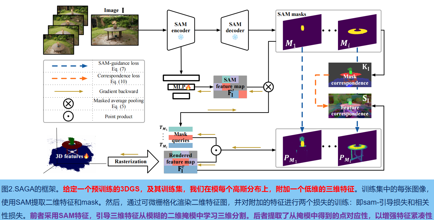
As shown in Figure 2, given a pre-trained 3DGS model G and its training set, we first use the encoder of SAM to extract the two-dimensional features of each image I∈R H×W : F I SAM ∈R Csam×H ×W and a set of multi-granularity masks M I SAM ; then according to the extracted mask, low-dimensional features f g ∈ R C of each Gaussian G are trained to aggregate cross-view consistent multi-granularity segmentation information ((C represents the feature dimension , size defaults to 32). To further improve the compactness of features, we get point-wise correspondences from the extracted masks and extract them as features (i.e., correlation loss).
In the inference stage, for the specific view of camera pose v 2 , a set of queries Q is generated according to the input prompt p, and then these queries are used to perform effective feature matching with the learned features to retrieve the three-dimensional Gaussian distribution of the corresponding target . In addition, we introduce an efficient post-processing operation to refine the retrieved 3D Gaussian distribution by exploiting the strong 3D prior provided by the point cloud-like structure of 3DGS .
3. Training Gaussian features
Training image I with pose v, render corresponding feature map F using pre-trained 3DGS model g:
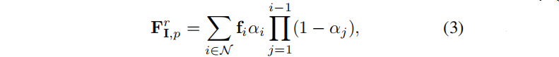
Among them, N is a set of overlapping ordered Gaussian distributions. During the training phase, except for the newly attached features, all other properties of the three-dimensional Gaussian G (such as mean, covariance and opacity) are frozen.
3.1 SAM-guidance Loss
2D mask MI automatically extracted by SAM is complex and confusing (i.e. a point in 3D space can be segmented into different objects/parts on different views). This ambiguous supervision signal poses a huge challenge to training 3D features from scratch. To solve this problem , we use SAM-generated features as guidance. As shown in Figure 2: Use MLP φ to project the SAM features into the same low-dimensional space as the three-dimensional features :

Then for each mask M extracted from M I SAM , after an average pooling operation, a corresponding query T M ∈ R C is obtained :

Among them, 'hollow 1' is the indicator function. Then use TM to segment the rendered feature map F I r by softmaxed :

Among them, σ represents the element-level sigmoid function. The SAM-guidance loss is defined as: the binary cross entropy between the segmentation result P M and the corresponding SAM extracted mask M:

3.2 Correspondence Loss
In practice, we found that the learned features of SAM-guided loss are not compact enough, reducing the quality of segmentation based on different cues (refer to the ablation study in Sec. 4). Inspired by previous contrastive correspondence distillation methods [9, 17], we introduce Correspondence loss to solve this problem.
As mentioned before, for each image I of height H and width W in the training set I, SAM is used to extract a set of masks M I . Considering two pixels p1, p2 in I, they may belong to many masks in M I. Let M I p1 and M I p2 respectively represent the masks to which pixel points p 1 and p 2 belong. If its IoU is larger, then the pixel features should be similar. Therefore, the correlation coefficient K I (p 1 , p 2 ) of mask :

The feature correlation S I (p 1 , p 2 ) between pixels p 1 , p 2 is defined as the cosine similarity between their rendered features:

correspondence loss (if two pixels never belong to the same part, reduce feature similarity by setting the 0 value in K I to −1.):

4. Inference
Although training is performed on rendered feature maps , the linearity of the rasterization operation (Equation 3) ensures that features in three-dimensional space are aligned with rendered features on the image plane . Therefore, 2D rendering features can be used to achieve three-dimensional Gaussian segmentation. This feature gives SAGA compatibility with various prompts. In addition, we also introduce an effective 3D prior post-processing algorithm based on 3DGS.
4.1 Point-based prompts
For the rendered feature map F v r of a specific view v , the corresponding features are directly retrieved to generate queries for positive and negative sample points. Let Q v p and Q v n represent N p positive queries and negative queries respectively. For the three-dimensional Gaussian g, its positive score S g p is defined as the maximum cosine similarity between its feature and the positive query, that is, max{ < f g , Q p > |Q p ∈Q v p } . Likewise, the negative fraction S g n is defined as max{ < f g , Q n > |Q n ∈Q v n } . Only when S g p > S g n does the three-dimensional Gaussian belong to the target G t . In order to further filter out the noisy Gaussian distribution, the adaptive threshold τ is set to a positive fraction, that is, g∈G t only if S g p > τ . τ is set to the average of the largest positive scores. Note that this filtering may result in many FN samples (positive samples not recognized), but this can be solved by post-processing in Section 4.5.
4.2 Tips based on Mask and Scribble
Simply treating dense hints as multiple points will result in huge GPU memory overhead. Therefore, we use the K-means algorithm to extract positive and negative queries from dense hints: Q v p and Q v n . As a rule of thumb, the number of clusters for Kmeans is 5 (can be adjusted according to the complexity of the target object).
4.3 SAM-based prompts
The preceding hints will be obtained from the rendered feature map. Due to SAM-guidance loss, we can directly use low-dimensional SAM features F' v to generate queries: first input the prompt into SAM to generate accurate 2D segmentation results M v ref . Using this 2D mask, we first obtain a query Q mask with mask average pooling , and use this query to segment the 2D rendered feature map F v r to obtain a temporary 2D segmentation mask M v temp , and then compared with M v ref . If the intersection of the two occupies the majority of the M v ref (90% by default), the Q v mask is accepted as the query. Otherwise, we use the K-means algorithm to extract another set of queries Q v kmeans from the low-dimensional SAM features F′ v within the mask . This strategy is adopted because the segmentation target may contain many components that cannot be captured by simply applying masked average pooling.
After obtaining the query set Q v SAM = {Q v mask } or Q v SAM = Q v kmeans , the subsequent process is the same as that of the previous prompt. We use dot product instead of cosine similarity as the measure of segmentation to accommodate the SAM-guided loss. For a three-dimensional Gaussian g, its positive score S g p is the maximum dot product calculated by the following query:

If the positive score is larger than another adaptive threshold τ SAM , then the three-dimensional Gaussian g belongs to the segmentation target G t , which is the sum of the mean and standard deviation of all scores.
5. Post-processing based on three-dimensional prior
There are two main problems in the initial segmentation G t of 3D Gaussians : (i) the problem of redundant noisy Gaussians, (ii) the omission of targets . To solve this problem, we use traditional point cloud segmentation techniques, including statistical filtering and region growing. For segmentation based on point and graffiti cues, statistical filtering is used to filter the noise Gaussian distribution. For mask prompts and SAM-based prompts, the 2D mask is projected onto G t to obtain a set of validated Gaussian functions, which are projected onto G to exclude unnecessary Gaussian functions. The resulting effective Gaussian function can be used as a seed for the region growing algorithm. Finally, a region growing method based on sphere query is adopted to retrieve all Gaussian functions required for the target from the original model G.
4.1 Statistical Filtering Statistical filtering
The distance between two Gaussian distributions can indicate whether they belong to the same target. Statistical filtering first uses the |-nearest neighbor (KNN) algorithm to calculate the nearest G t \sqrt{Gt} of each Gaussian distribution in the segmentation result GtGtThe mean distance of a Gaussian distribution. Subsequently, we calculated the mean (µ) and standard deviation (σ) of these average distances for all Gaussians in G t . We then remove Gaussian distributions whose mean distance exceeds µ+σ and obtain G t' .
4.2 Filtering based on regional growth
The 2D mask from the mask cue or the sam-based cue can be used as a prior to accurately locate the target : first, the mask is projected onto the coarse Gaussian result Gt , resulting in a Gaussian subset, denoted as Gc . Subsequently, for each Gaussian g within G c , the Euclidean distance d g of the nearest neighbor in the subset is calculated :

In the formula, D() represents the Euclidean distance. Then, adjacent Gaussians (distances smaller than the maximum nearest neighbor distance in the set G c ) are iteratively added to the coarse Gaussian result G t . This distance is formalized as: Note that although point cues and scribble cues can also roughly locate the target, growing the area based on them is time-consuming. Therefore, we only use it when there is a mask.
4.3 Growth based on Ball Query
The filtered segmentation output G′ t , may lack all Gaussians of the target. To solve this problem, we use the ball query algorithm to retrieve all required Gaussians from all Gaussians G. Specifically, this is achieved by examining a spherical neighborhood of radius r. The Gaussian distributions located within these spherical boundaries in G are then aggregated into the final segmentation result G s . The radius r is set to the maximum nearest neighbor distance in G' t :

4. Experiment
1.Dataset
Quantitative experiments, using Neural Volumetric Object Selection (NVOS), SPIn-NeRF [33] data set. The NVOS dataset is based on the LLFF dataset, which includes several forward scenarios. For each scene, the NVOS dataset provides a reference view with scribbles and a target view annotated with 2D segmentation masks. Similarly, the SPIn-NeRF [33] dataset also manually annotates some data based on the widely used NeRF dataset [11, 24, 26, 31, 32]. In addition, we also annotated some objects in the LERF-Figurine scene using SA3D to demonstrate the better trade-off of SAGA in terms of efficiency and segmentation quality.
For qualitative analysis, LLFF, MIP-360, T&T data set and LERF data set were used.
2. Quantitative experiment
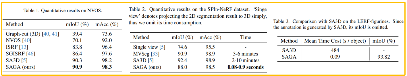
NVOS : Follows SA3D [5] to process graffiti provided by the NVOS dataset to meet the requirements of SAM. As shown in Table 1, SAGA is the same as the previous SOTA SA3D and significantly outperforms the previous feature imitation-based methods (ISRF and SGISRF), which demonstrates its fine-grained segmentation capabilities.
SPIn-NeRF : Evaluation follows SPIn-NeRF, which specifies a view with a 2D ground truth mask and propagates this mask to other views to check the accuracy of the mask. This operation can be thought of as a masking prompt. The results are shown in Table 2. MVSeg uses the video segmentation method [4] to segment multi-view images, and SA3D automatically queries the two-dimensional segmentation basic model of the rendered image on the training view. Both require proposing a 2D segmentation model many times. Remarkably, SAGA shows comparable performance to them nearly one thousandth of the time. Note that the slight degradation is caused by the suboptimal geometry learned by 3DGS.
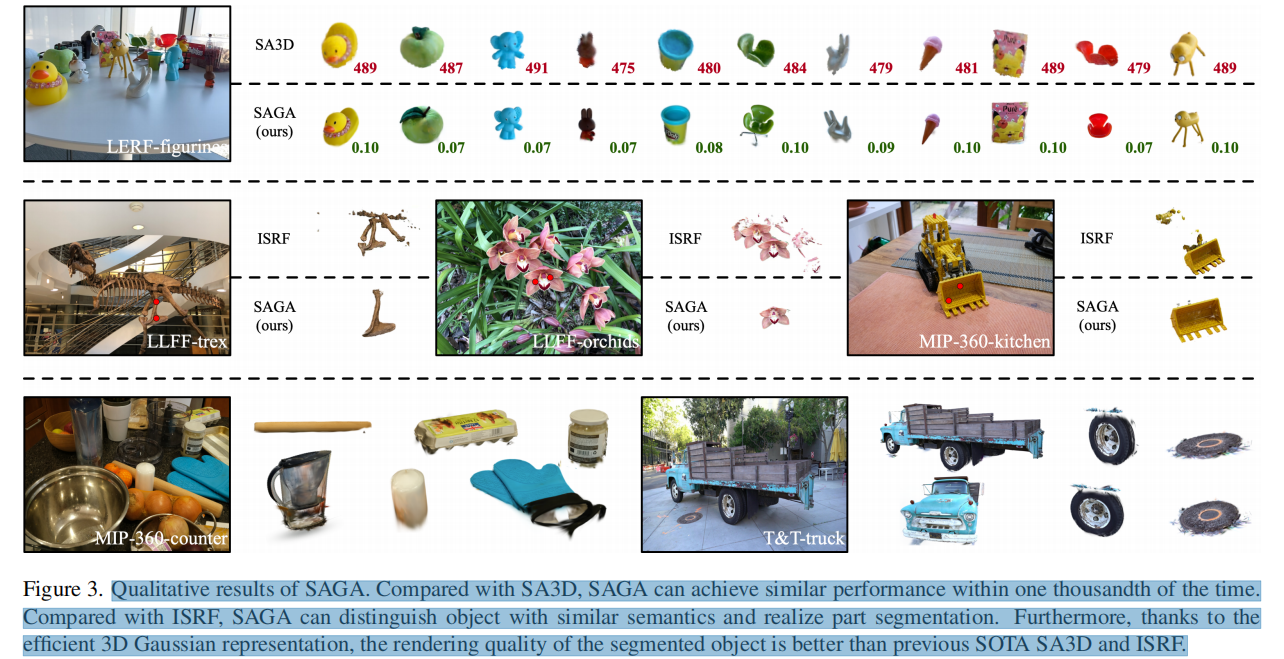
Comparison with SA3D . Run SA3D based on the LERF-futtes scene to obtain a set of annotations for many objects. Subsequently, we use SAGA to segment the same objects and check the IoU and time cost of each object. The results are shown in Table 3, and we also provide visualization results comparing with SA3D. It is worth noting that the training resolution of SAGA is much higher due to the huge GPU memory cost of SA3D. This shows that SAGA can obtain higher quality 3D assets in less time. Even taking into account the training time (~10 minutes per scene), the average segmentation time per object in SAGA is much smaller than that of SA3D.
3. Qualitative experiment
4. Failure cases
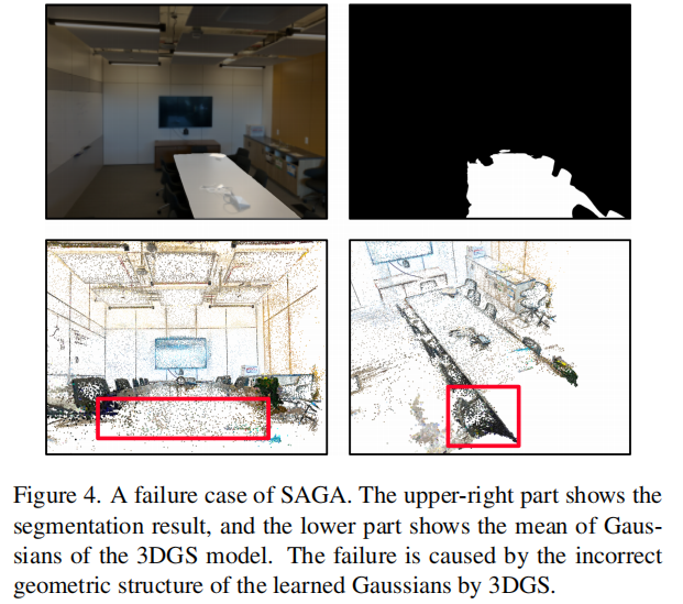
In Table 2, SAGA exhibits suboptimal performance compared to previous methods. This is because the segmentation of the LLFF-room scene fails, revealing the limitations of SAGA. We show in Figure 4 the average of the colored Gaussian functions, which can be viewed as a kind of point cloud. SAGA is susceptible to insufficient geometric reconstruction of 3DGS models . As shown in the red box, the table's Gaussians are significantly sparse, with the Gaussians representing the table's surface floating below the actual surface. To make matters worse, the Gaussian on the chair is very close to the person on the table. These problems not only hinder the learning of discriminative 3D features but also affect the effectiveness of post-processing. We believe that improving the geometric fidelity of 3DGS models can improve this problem.
d \sqrt{d}d 1 0.24 \frac {1}{0.24} 0.241 x ˉ \bar{x} xˉ x ^ \hat{x} x^ x ~ \tilde{x} x~ ϵ \epsilonϵ
Summarize
提示:这里对文章进行总结:
For example: The above is what I will talk about today. This article only briefly introduces the use of pandas, and pandas provides a large number of functions and methods that allow us to process data quickly and conveniently.