
1. Introduction
In time series analysis, it is often necessary to understand the trend direction of a series by considering previous values. Approximation of the next value in the sequence can be performed in a variety of ways, including using a simple baseline or building an advanced machine learning model.
The exponential (weighted) moving average is a robust trade-off between these two methods. There is a simple recursive method behind the scenes that implements this algorithm efficiently. At the same time, it is very flexible and can be successfully adapted to most types of sequences.
This article presents the motivation behind the approach, its workflow, and a description of bias correction—an effective technique for overcoming bias barriers in approximations.
2. Motive
Imagine a problem of approximating a given parameter that changes over time. At each iteration, we know all the values before it. The goal is to predict the next value based on the previous value.
A naive strategy is to simply take the average of the last few values. This may work in some cases, but is less suitable where the parameters are more dependent on the latest value.
One of the possible ways to overcome this problem is to assign higher weight to newer values and less weight to previous values. Exponential Moving Average is a strategy that follows this principle. It is based on the assumption that newer values of a variable contribute more to the formation of the next value than previous values .
3. Formula
To understand how the exponential moving average works, let’s look at its recurrence equation:

exponential moving average formula
- vₜ is a time series that approximates a given variable. Its index t corresponds to timestamp t. Since the formula is recursive, it requires the value v₀ for the initial timestamp t = 0. In practice, v₀ usually takes 0.
- θ is the observation value of the current iteration.
- β is a hyperparameter between 0 and 1 that defines how the weight importance should be distributed between the previous mean vₜ-₁ and the current observation θ
Let's write this formula for the first few parameter values:

The formula for obtaining the t-th timestamp
As a result, the final formula looks like this:

Exponential moving average of the t timestamp
We can see that the most recent observation θ has a weight of 1, the second to last observation — β, the third to last — β², etc. Since 0 < β < 1, the multiplicative term βᵏ decreases exponentially with increasing k, so the older the observations, the less important they are . Finally, multiply each sum term by (1 - β).
In practice, the value of β is usually chosen close to 0.9.
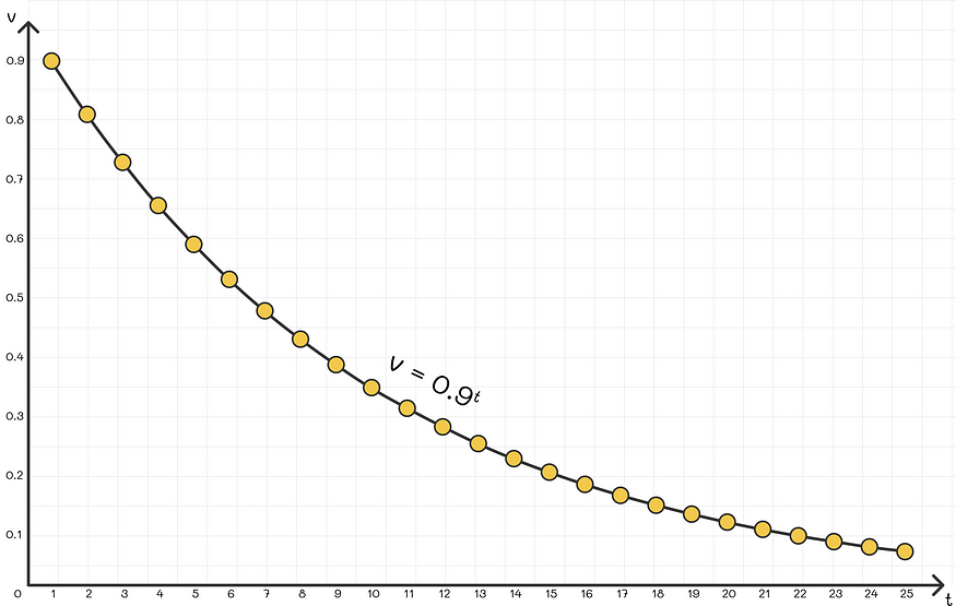
Weight distribution for different timestamps (β = 0.9)
4. Mathematical explanation
Using the famous second fantastic limit in mathematical analysis, the following limit can be proven:

By replacing β = 1 - x , we can rewrite it as:

We also know that in the equation for the exponential moving average, each observation is multiplied by the term βᵏ, where k represents the timestamp before the observation was calculated. Since the base β is equal in both cases, we can make the exponents of the two formulas equal:
By using this equation, for a selected value of β, we can calculate the approximate number of timestamps t required for the weight term to reach the value 1/e ≈ 0.368. This means that observations computed in the last t iterations have weight terms greater than 1/e, while more precedent weight terms computed in the last t timestamp range have less importance than 1/e. Much smaller.
In practice, weights below 1/e have little effect on the exponentially weighted average. This is why it is said that for a given value of β, the exponentially weighted average takes into account the last t = 1 / (1 - β) observations .
To better understand this formula, let us substitute different values for β :

For example, taking β = 0.9 means that approximately in t = 10 iterations, the weight decays to 1/e compared to the weight of the current observation. In other words, the exponentially weighted average mainly depends on the last t = 10 observations.
5. Deviation calibration
A common problem with using exponentially weighted average is that in most problems it does not approximate the first series value very well. This happens because there is not enough data in the first iteration. For example, assume we are given the following time series:
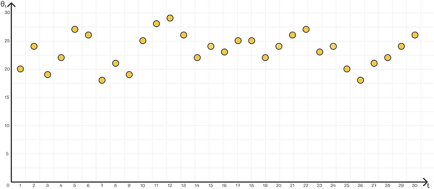
The goal is to approximate it with an exponentially weighted average. However, if we use the normal formula, then the first few values will put a lot of weight on v₀, which is 0, while most points on the scatter plot will be above 20. Therefore, the first weighted average of the sequence will be too low an accurate approximation of the original sequence.
One simple solution is to use a v0 value close to the first observation θ1. Although this method works well in some cases, it is still not perfect, especially if the given sequence is unstable. For example, if θ2 is too different from θ1, the weighted average will usually give more weight to the previous trend v1 than the current observation θ2 when calculating the second value v2. As a result, the approximation will be very poor.
A more flexible solution is to use a technique called " bias correction ." Instead of simply using the calculated value vₖ, they divide by (1 —βᵏ). Assuming that β is chosen close to 0.9-1, this expression tends to be close to 0 for the first iteration with smaller k. So now instead of slowly accumulating the first few values of v₀ = 0, we divide them by relatively small numbers, scaling them to larger values.
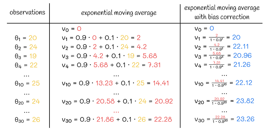
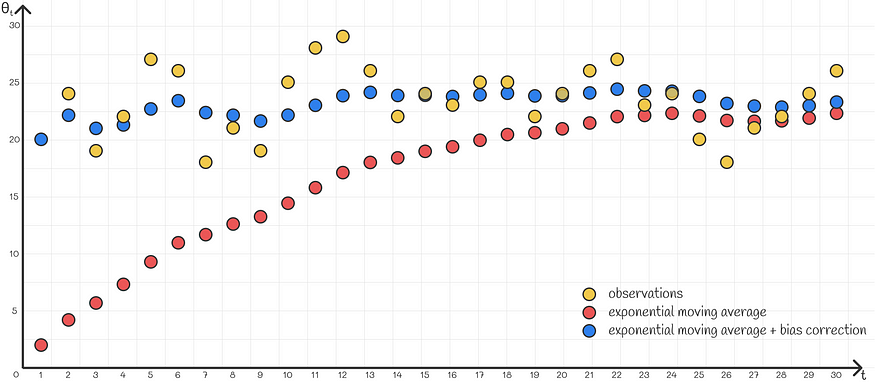
Exponential moving average calculation example with and without bias correction
In general this scaling works very well and adapts the first few items exactly. As k becomes larger, the denominator gradually approaches 1, gradually neglecting the effect of such scaling which is no longer needed, since starting from a certain iteration the algorithm can rely on its most recent values with high confidence without any additional scaling.
6. Conclusion
In this article, we introduce a very useful technique for approximating time series sequences. The robustness of the exponentially weighted average algorithm is mainly achieved through its hyperparameter β, which can be adapted to specific types of sequences. In addition to this, the introduced bias correction mechanism allows efficient approximation of data even on early timestamps with too little information.
Exponentially weighted average has a wide range of applications in time series analysis. Additionally, it is used in variations of the gradient descent algorithm to speed up convergence. One of the most popular is the momentum optimizer in deep learning, which eliminates unnecessary oscillations of the optimized function, aligning it more precisely with local minima.