Classic works, worth reading, English original download link[Free] Modern Radar for Automotive Applications resources-CSDN library.
2.5 检测基础
For radar measurements to test the presence of a target, one of the following two assumptions can be assumed to be true:
•H0:—The measurement result is only noise.
•H1:—The measurement is the comprehensive result of noise and target echo.
The radar system’s detection logic examines each measurement and selects a hypothesis as the best metric for the measurement. If H0 is selected, the system declares that the measurement comes entirely from noise and the target does not exist. On the other hand, if H1 is selected, the radar system declares that the target is present.
The probability density function (pdf) can be used to analyze signals. Two probability density functions, py (y|H0) and py (y|H1), define the H0 and H1 hypotheses respectively. y is the measurement sample to be tested. py (y|H 0) is the probability density function of y when the target does not exist, and py (y|H1) is the probability density function of y when the target exists. Based on these two probability density functions, the following probabilities can be defined:
•Probability of Detection (PD): The probability that the radar system claims to have detected the target when the target is actually present (choice H1).
•Probability of False Alarm (PFA): The probability that the radar system claims to have detected a target (select H1), but the target does not actually exist.
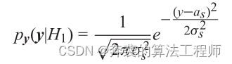
In order to further discuss how to use PD and PFA to characterize radar systems, consider that the noise of the radar system is white noise and py (y|H0) is a normal distribution. In addition, considering that the target is non-undulating, py (y| H1) is also a normal distribution, because H1 is a combination of noise and target echo.
![]() (2.80)
(2.80)
![]() (2.81)
(2.81)
Here![]() and
and ![]() are the average amplitudes of hypothetical H0 and H1 respectively.
are the average amplitudes of hypothetical H0 and H1 respectively. ![]() and
and ![]() are the variances of H0 and H1 respectively. Therefore, the probability density function is:
are the variances of H0 and H1 respectively. Therefore, the probability density function is:
 (2.82)
 (2.83)
Figure 2.16 draws these two probability density functions, py (y|H0) and py (y|H1). In radar systems, it is more commonly used to use the Neyman-Pearson criterion. Under the constraint that the false alarm probability PFA does not exceed a constant, a threshold T is selected to maximize the detection probability PD. As shown in Figure 2.16, PFA is the area above the threshold T in py (y|H0) (blue shade), which can be calculated by the following formula:
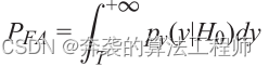 (2.84)
PD is the area above the threshold T in py (y|H1) (red shade):
 (2.85)
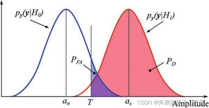
Figure 2.16 Probability density function assuming H0 and H1
It should be noted that as long as the threshold T is selected, the PFA remains unchanged. However, PD changes with the signal-to-noise ratio SNR, which is![]() in Figure 2.16. PD increases with the increase of signal-to-noise ratio, as shown in Figure 2.17, where PFA=1×10⁻⁶. Coherent processing means taking phase information into account, while incoherent processing discards phase information. Figure 2.18 shows the PD versus PFA plot when the signal-to-noise ratio is 10 dB.
in Figure 2.16. PD increases with the increase of signal-to-noise ratio, as shown in Figure 2.17, where PFA=1×10⁻⁶. Coherent processing means taking phase information into account, while incoherent processing discards phase information. Figure 2.18 shows the PD versus PFA plot when the signal-to-noise ratio is 10 dB.
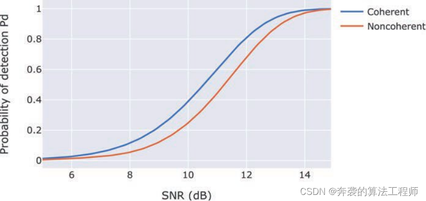
Figure 2.17 Relationship between detection probability and SNR, PFA=1×10⁻⁶
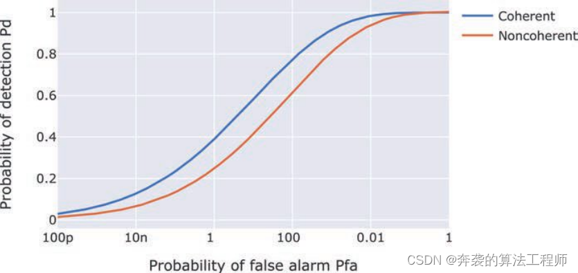
Figure 2.18 Relationship between detection probability and false alarm probability, SNR=10dB
2.5.1 Coherent and incoherent accumulation
Accumulation is one of the commonly used techniques in radar signal processing to improve the signal-to-noise ratio. Both coherent and incoherent accumulation have wide applications. Coherent accumulation refers to the accumulation of complex data, and non-coherent accumulation refers to the accumulation based only on data size. It can be seen from Figure 2.17 and Figure 2.18 that even if accumulation is not performed, there will be a small loss of signal-to-noise ratio when discarding the phase during processing.
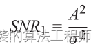
Coherent accumulation is beneficial to improving the signal-to-noise ratio. However, it also requires more processing since it needs to handle complex data. Assume that the radar receives measurements from the target's echo![]() , where A is the amplitude, ϕ is the phase, and ω is additive noise with power σ2. The signal-to-noise ratio is defined as
, where A is the amplitude, ϕ is the phase, and ω is additive noise with power σ2. The signal-to-noise ratio is defined as
 (2.86)
Assuming that the measurement has been performed N times, there may be N channels taking the same measurement or repeating the measurement N times. For repeated measurements, the echo response is expected to be the same, but the noise is independent each time. Therefore, phase information can be added to all measurements.
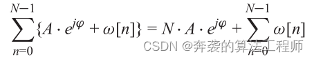 (2.87)
The power of the accumulated signal part is N2 *A2. For the independent noise part, the total noise power is the sum of the individual noise powers, which is N*σ2. The comprehensive signal-to-noise ratio is:
 (2.88)
The number of accumulation times N is also called the coherent accumulation gain. For coherent accumulation, it is assumed that the phase of the signal part remains the same across multiple measurements. However,this is not always the casein reality. In most cases, the signal needs to be preprocessed to make the phase consistent for each measurement. This process also requires additional coherent accumulation calculations. When PFA = 1 * 10 -6, the relationship between PD, signal-to-noise ratio, and accumulation N is shown in Figure 2.19.
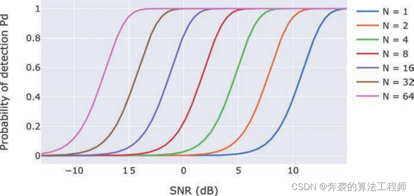
Figure 2.19 The relationship between PD and coherent accumulation signal-to-noise ratio when PFA = 1 * 10 -6
Consider the incoherent accumulation of a non-fluctuating target, also known as a "Swerling 0" or "Swerling V" target, with Gaussian white noise ω. For simplicity, assume the total power of ω is 1. Assume that under H0, the target does not exist, and the probability density function of y=|ω| follows the Rayleigh distribution.
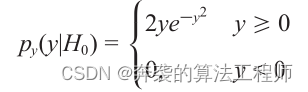 (2.89)
Assume that under H1, ![]() is a Rice distribution:
is a Rice distribution:
 (2.90)
Here![]() is the modified Bessel function of the first kind of order 0.
is the modified Bessel function of the first kind of order 0.
By performing non-coherent accumulation of N (N> 1) samples, the probability distribution under the H0 hypothesis is obtained as the Erlang distribution.
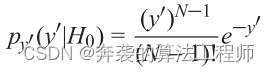 (2.91)
Assume that the probability density function under H1 is:
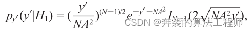 (2.92)
Here![]() is used as a square law detector.
is used as a square law detector.
The detailed derivation of these equations is not presented in this chapter as it is beyond the scope of this book. To better understand non-coherent accumulation, Figure 2.20 and Figure 2.21 provide a simple illustration of the effect of non-coherent accumulation. In both Figure 2.20 and Figure 2.21, the unaccumulated raw signal-to-noise ratio is 4 (6 dB). Figure 2.20 and Figure 2.21 are the cases of N= 2 and N= 10 respectively. In order to calculate the accumulated signal-to-noise ratio, the mean of all probability density distributions needs to be calculated. For the Erlang distribution in (2.91), the mean is μH0 = N. For the distribution in equation (2.93), the mean can be calculated through numerical methods:
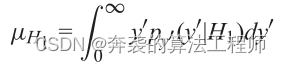 (2.93)

Figure 2.20 Probability density function of H0 and H1 for 2 measured incoherent accumulations
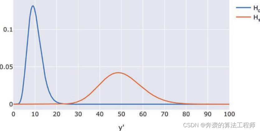
Figure 2.21 Probability density function of H0 and H1 for incoherently accumulated 10 measurements
对于图2.20中N=2,![]() ,
,![]() ,
,
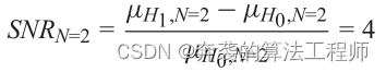 (2.94)
For the example in Figure 2.21, N=10,![]() ,
,![]()
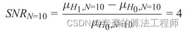 (2.95)
Therefore, non-coherent accumulation cannot actually improve the signal-to-noise ratio.
Now consider PFA with different values of N. It is difficult to derive the threshold T analytically based on PFA and (2.91). A simpler approach is to numerically calculate the integral of p y ‘ (y ‘|H 0) as follows:
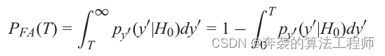 (2.96)
Figure 2.22 shows the relationship between PFA and the normalized threshold T’ when N= 2 and N= 10. The threshold is normalized to the mean of the probability density function in (2.89) for better comparison. For N= 2, T’ = 5.9 gives 10 -4, on the other hand, to get the same PFA, in the case of N= 10 T’ = 2.6. Therefore,for non-coherent accumulation, effective gain< is achieved by lowering the threshold of somePFA a i=4>. In other words, with more accumulation, the same PFA can be achieved with a lower threshold, and the minimum signal-to-noise ratio required for the target to be detected is also reduced.
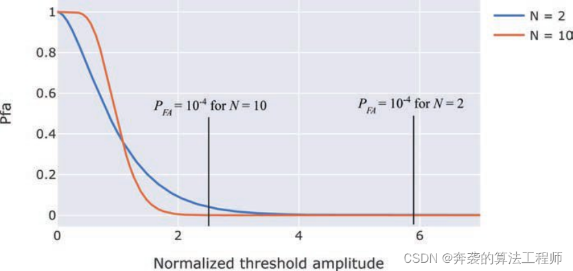
Figure 2.22 Relationship between PFA and normalized threshold under different accumulation values
The previous analysis only considered the non-fluctuating target, that is, the case of "Swerling 0" or "Swerling V". A more realistic scenario would be the ups and downs targets mentioned above, including the "Swerling I, II, III and IV" models. The derivation of probability density functions for undulating targets is beyond the scope of this book.
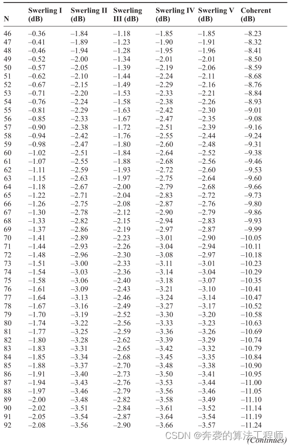
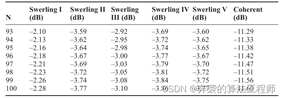
Popular signal processing tools, such as MATLAB®, have convenient functions to perform this analysis. Figures 2.23 and 2.24 show the relationship between the PD and the incoherent accumulation signal-to-noise ratio of the Swerling I, II, III, IV and V models under the condition of PFA = 1 * 10 -6. (Table 2.6)
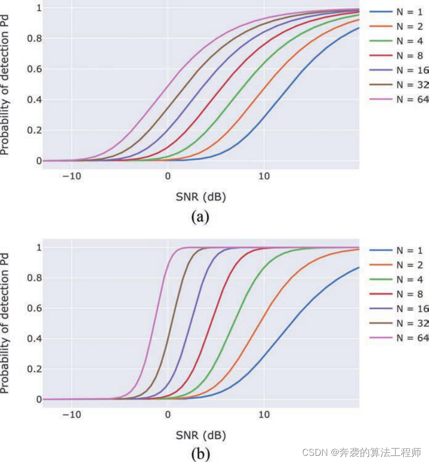
Figure 2.23 The relationship between PD and incoherent accumulation signal-to-noise ratio when PFA = 1 * 10 -6
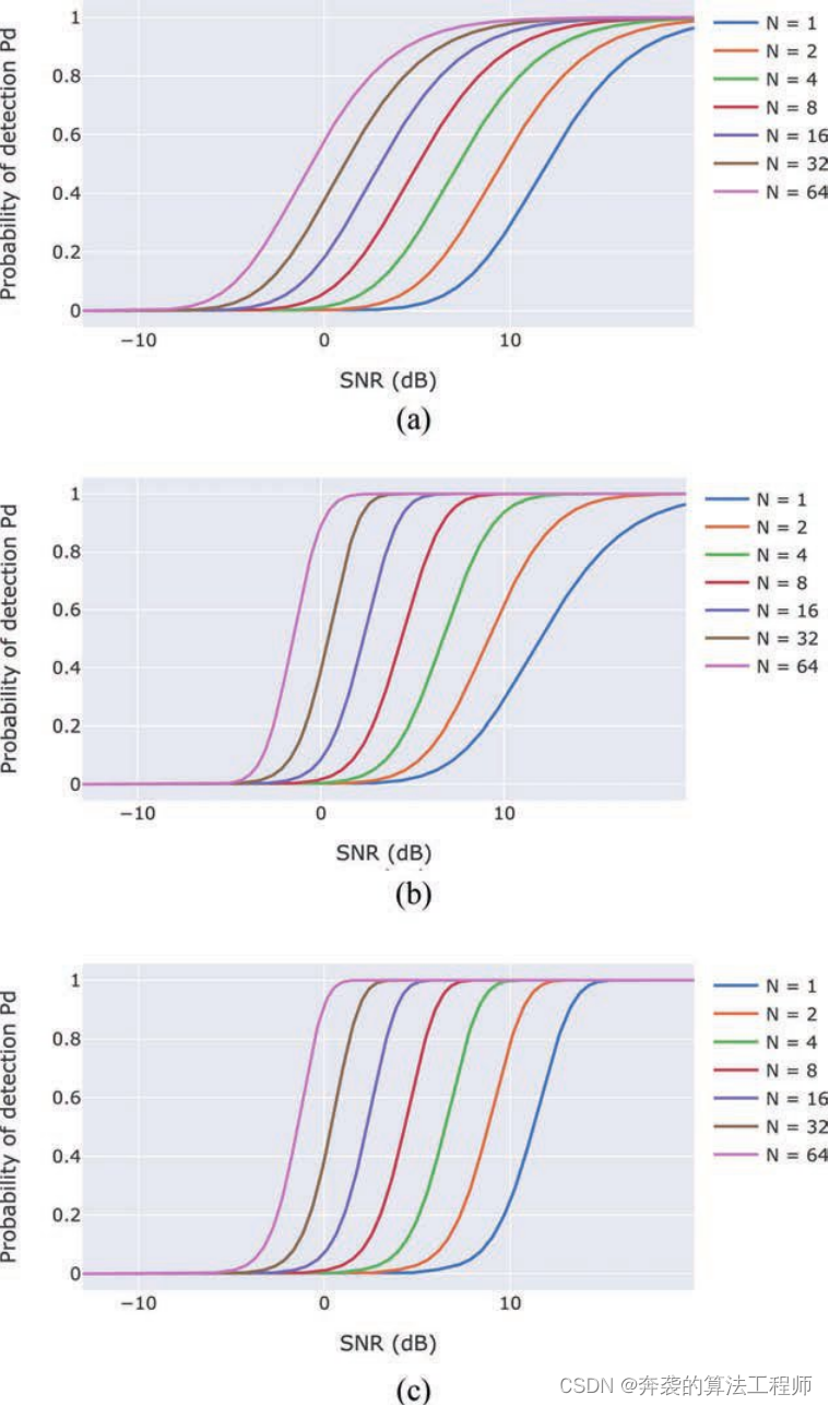
Figure 2.24 The relationship between PD and incoherent accumulation signal-to-noise ratio when PFA = 1 * 10 -6
2.5.2Determine the minimum signal-to-noise ratio of detection probability and false alarm probability
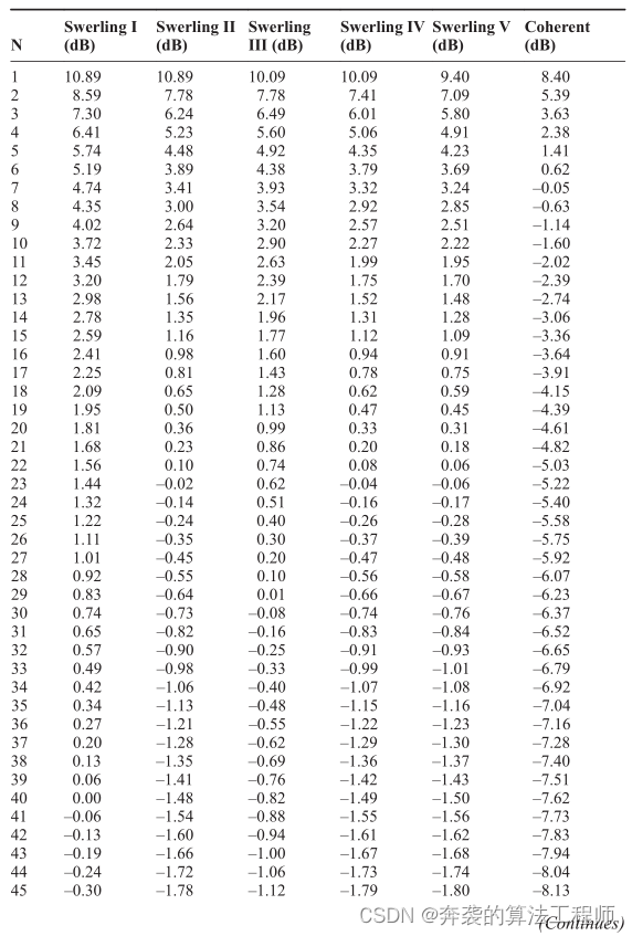
The relationship between PD and PFA has been discussed in the previous content. For a certain PFA, a threshold can be obtained from py’ (y’|H0), which is the probability density function (PDF) of target-free echo noise. Another threshold can also be obtained from p y' (y'|H1), which is based on the noisy target echo PDF value of a certain PD. Usually the two thresholds are separated, and their difference increases with the signal-to-noise ratio. decreases. Under a certain signal-to-noise ratio, these two thresholds are equal to each other. This signal-to-noise ratio is the minimum signal-to-noise ratio required to meet the predefined PD and PFA. In the case of accumulation, the difference between the minimum signal-to-noise ratios after accumulation is equal to the accumulation gain. Table 2.6 gives the minimum signal-to-noise ratio required for PFA = 10 -4 and PD = 0.5 under different target models and accumulation types.
. For example, using radar in an emergency braking system requires the detection of pedestrians with PD = 0.5 and PFA = 10-4 within R0 distance. Pedestrians are typically classified as "Swerling I" targets, with typical RCS around -10dBsm. From Table 2.6, it can be seen that the required minimum signal-to-noise ratio is 10.89 dB. Therefore, for a target of -10dBsm, the radar needs to be designed to have a signal-to-noise ratio of at least 10.89dB within the R0 distance. If the radar is designed to non-coherently accumulate 8 channels during processing, the required minimum signal-to-noise ratio can be relaxed to 4.35 dB. The signal-to-noise ratio difference 10.89 ~ 4.35 = 6.54 dB is the incoherent accumulation gain of the Swerling I target.
Table 2.6 Minimum signal-to-noise ratio for PFA = 1 * 10 -4, PD=0.5
2.5.3Constant false alarm rate detection
As mentioned above, standard radar threshold detection assumes that the noise level at the receiver is known and stable. Therefore, accurate thresholds can be obtained to guarantee the specified PFA. However, in the real world, noise levels vary with a variety of factors, including environment, temperature, and component aging. Radar systems need to estimate the noise level from measurements and derive thresholds on this basis. Temperature compensation and periodic recalibration can partially solve the problem of noise power variation; however, these methods are not practical in high-volume production for automotive applications. In addition, automotive radars are often exposed to complex electromagnetic environments and are interfered by radars from surrounding vehicles. Strong interference can significantly increase noise power. Therefore, adaptive calculation of automotive radar noise power has always been necessary.
Constant False Alarm Rate (CFAR) detection, also known as “adaptive threshold detection” or “auto-detection”, is a set of techniques designed to provide predictable detection and false alarm behavior in realistic noise scenarios. For CFAR detection, the actual noise power must be estimated from the data in real time in order to adjust the detector threshold to maintain the ideal PFA. Various CFAR algorithms from simple to complex have been reported. In order to provide a basic impression of CFAR detection, this section will briefly discuss two basic CFAR algorithms, namely unit-averaged CFAR (CA-CFAR) and ordered statistical CFAR (OS-CFAR).
2.5.3.1 CA-CFAR
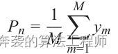
CA-CFAR is one of the most basic CFAR algorithms. It is also used as a baseline comparison for other CFAR techniques. Figure 2.25 shows the sliding window processing structure of one-dimensional CA-CFAR, which can also be calculated in two-dimensional range Doppler images, as shown in Figure 2.26. Noise samples are extracted from leading and lagging units (training units) surrounding the unit under test (CUT). The protection unit is placed near the CUT. The purpose of these guard units is to avoid signal components leaking into the training units and thus adversely affecting the noise estimate. The noise power Pn can be calculated as
 (2.97)
Where M is the number of training units, ym is the power of the Mth training unit. The number of training units and protection units can be adjusted as needed. The threshold T is given by
![]() (2.98)
(2.98)
Among them, the scale factor α is called the threshold factor. The value of α is calculated based on the expected false alarm rate PFA and (2.96). If there is no pulse accumulation, it can be obtained by the following formula:
![]() (2.99)
(2.99)
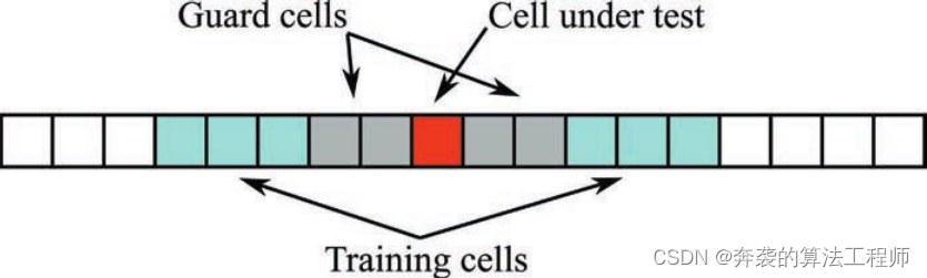
Figure 2.25 One-dimensional CA-CFAR processing
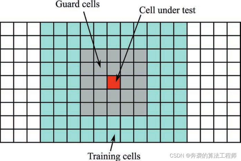
Figure 2.26 Two-dimensional CA-CFAR processing
Figure 2.27 shows the working principle of CA-CFAR in FMCW radar. There were two targets in the trial, 95 meters and 30 meters. CA-CFAR uses two protection units and 10 trailing units, PFA = 10-2. As can be seen from Figure 2.27, the CA-CFAR threshold has a high shoulder near the target peak, which means that in addition to large targets, smaller targets will be masked by the threshold. Therefore, CA- CFARneeds to assume that targets need to be isolated, and that targets need to be isolated far enough so that they are not obscured by the shoulders of other targets< /span>. Another assumption of CA-CFAR is that the noise of the training units is independent and uniformly distributed.
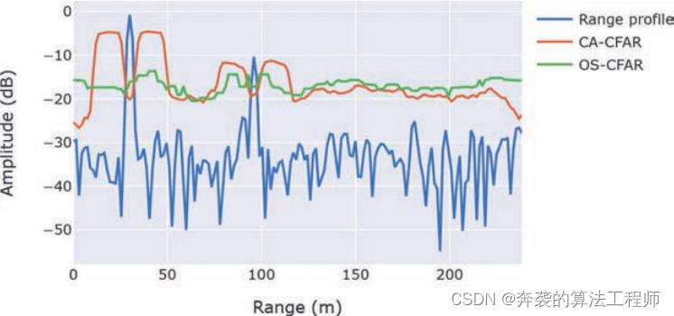
Figure 2.27 CA-CFAR and OS-CFAR performance examples
Due to the performance limitations of CA-CFAR, many extensions to CA-CFAR have been caused, such as the smallest unit average CFAR and the larger unit average CFAR.
2.5.3.2 OS-CFAR
OS-CFAR is another range-based method of CFAR threshold. OS-CFAR uses a one-dimensional or two-dimensional sliding window structure similar to CA-CFAR, as shown in Figures 2.25 and 2.26. Protection units can be used if necessary. Different from CA-CFAR, OS-CFAR sorts the data samples [y 1, y 2, ..., yM] in the training unit to form a new ascending sequence, represented as [y (1), y (2), ... ,y(M)]. Then, select the k-th element in the ordered list as a representative of the noise level and set a threshold that is a multiple of that value:
![]() (2.100)
(2.100)
For the calculation of αOS, please refer to the literature [29]. Noise is estimated from only one data sample, not the average of all data samples. However, since the samples used are determined based on all data samples, the threshold actually utilizes the information of all samples.
Figure 2.27 shows the working principle of OS-CFAR in FMCW radar; M= 20, k = 15, PFA= 10-2. It can be seen that OS-CFAR does not have high shoulders around the target peak. The main disadvantage of OS-CFAR is that executing the sorting algorithm requires high processing power, and this processing power must be provided in the real-time part of the radar signal processing.