Factor graph optimization principle (iSAM, iSAM2)
slam problem
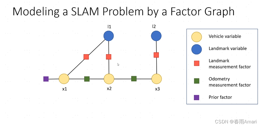
Before introducing the factor graph, let’s start with a simple slam problem, as shown in the following figure:
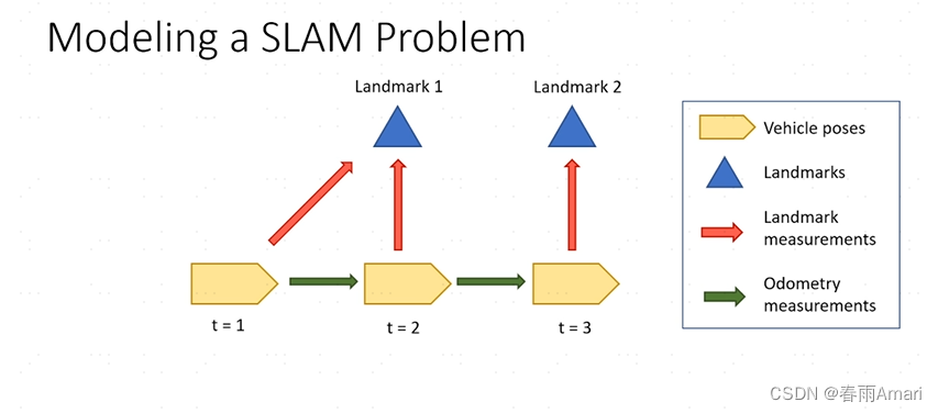
The figure clearly shows the relationship between each node and the edges connecting the nodes. The definition of space is not explained too much about the graph structure, and it is assumed that readers already have certain prior knowledge. In the slam problem shown above, the problem we actually want to solve is to recover the robot's path and environment map from the robot's control and observation.
Modeling the slam problem via Bayesian networks
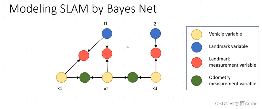
In the Bayesian network, variables are connected through directed edges. In addition to the landmark state node and the robot's state node (the two state nodes are state variables), the landmark observation node (red) and motion are also defined. Observation nodes (green) (the two observation nodes are observation variables). This Bayesian actually describes a joint probability model of states and observations. Assuming that the state variables of the system ), that is, if the state quantity of the robot and the sensor model are known, the observation quantity of the robot can be calculated. Therefore, a generative model is obtained as shown in the figure below:
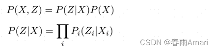
Since the observations are independent of each other, the model described in the following formula can be obtained:
From Bayesian networks to factor graphs
Based on the above, we know that the Bayesian network is a generative model that solves the problem of obtaining observed variables from state variables, and our problem is to deduce state variables from observed variables, which is a state estimation problem. This This leads to the factor graph, which is an inference model.
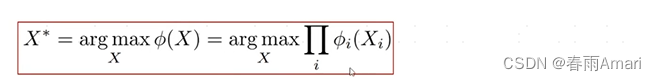
First, let’s make a derivation of the problem: Since we need to deduce the state quantity from the observation quantity, this is a posterior probability problem. Combined with Bayesian Dingling, the problem is described as maximizing a posterior probability Experimental probability problem (MAP), that is, given the system observation quantity, solve the system state quantity so that the conditional probability of the following formula is maximized:
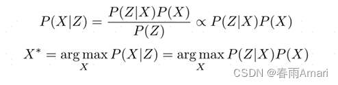
Through the above definition, the MAP problem is converted into solving an optimal The state maximizes the product of likelihood probability and prior probability.
Derivation of the definition of factors: factorize the prior and likelihood terms as factors:
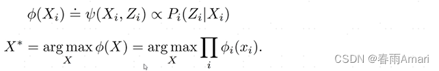
Express each term in the above product form as a factor, and express the state variables as nodes , the observed quantities are expressed as edges, which are transformed into the following factor graph.
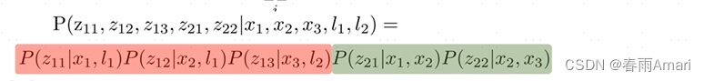
For the above factor diagram, we use the following formula to describe it:

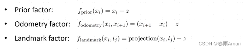
The red part represents the observation factor, the green part is the odometry factor, and the purple part is the first test factor. So what is the problem we want to solve, which is to find an optimal X that maximizes the product of these factor graphs.

The definition of each factor in the factor diagram: In the factor diagram, each factor is usually defined in the form of an exponential function. This is because the observations we obtain have uncertainties. , and in reality this uncertainty usually obeys Gaussian distribution:
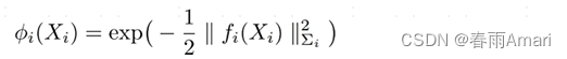
where f(x) represents the error function. When the error is smaller, the exponential function is larger, and its definition As shown in the figure below:
Through the above explanation, here we finally get the problem we want to solve after defining the factor graph. Let’s go through it first. First, we introduced the Bayesian network, which is a probabilistic network. The Bayesian network can solve the problem of deriving observed variables from known state variables. But the fact is that we can usually get the observed variables. If we want State variables were derived, so we derived the factor graph, and combined with Bayes' theorem, described the problem as a maximum posterior probability problem. Finally, the objective function is obtained:
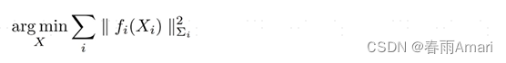
Now that we have the objective function, the last remaining question is how to solve this optimization problem. By taking the negative logarithm of the right side of the objective function, the problem of maximizing the factor can be transformed into a nonlinear least squares problem:
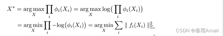
By solving this nonlinear least squares problem, we can get The optimal solution to the problem.
Solving nonlinear least squares problems
For the least squares problem of the above formula, it can be solved by Gauss-Newton iteration method. First, an initial value of X), find a modified amount based on the given variable, and finally use this initial value plus this modified amount to get the new state X, and repeat the iterative process until convergence. The process is shown in the figure below:
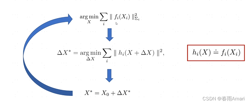
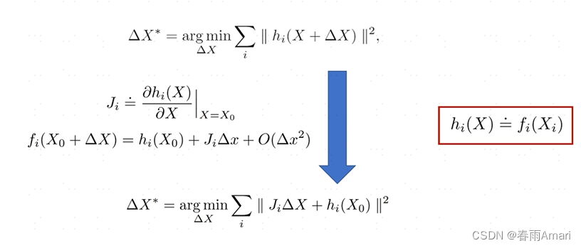
For the nonlinear least squares problem in the figure above, perform a first-order Taylor expansion on the middle formula to convert it into a linear least squares problem. :
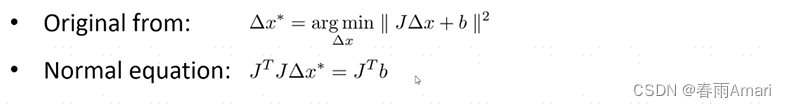
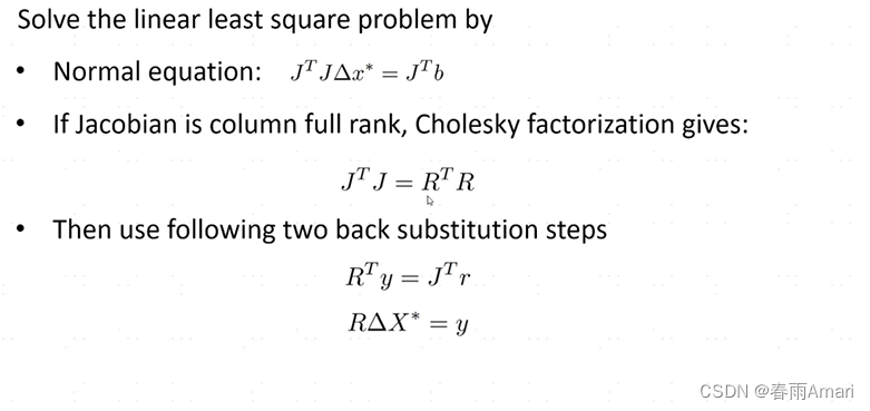
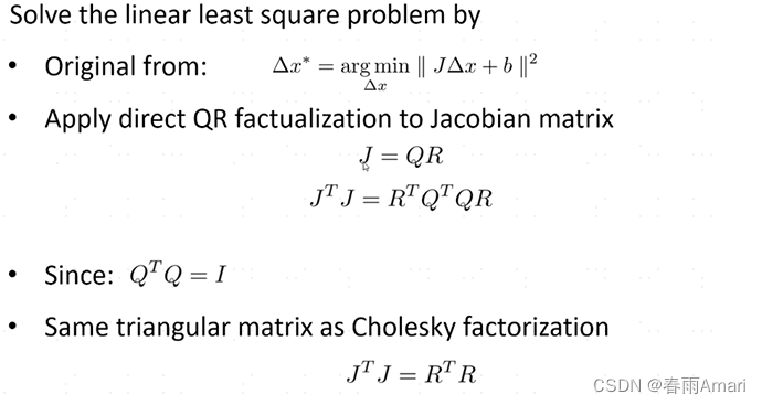
The current problem is transformed into how to solve this linear least squares problem. For a linear least squares problem, a relatively mature method is used to obtain the optimal solution to the linear minimum problem. , the more common method is Normal equation:
The Normal equation problem can be solved through Cholesky decomposition:
It can also be solved by QR decomposition:
Let’s illustrate the solution process of the factor graph through the simple slam problem at the beginning:
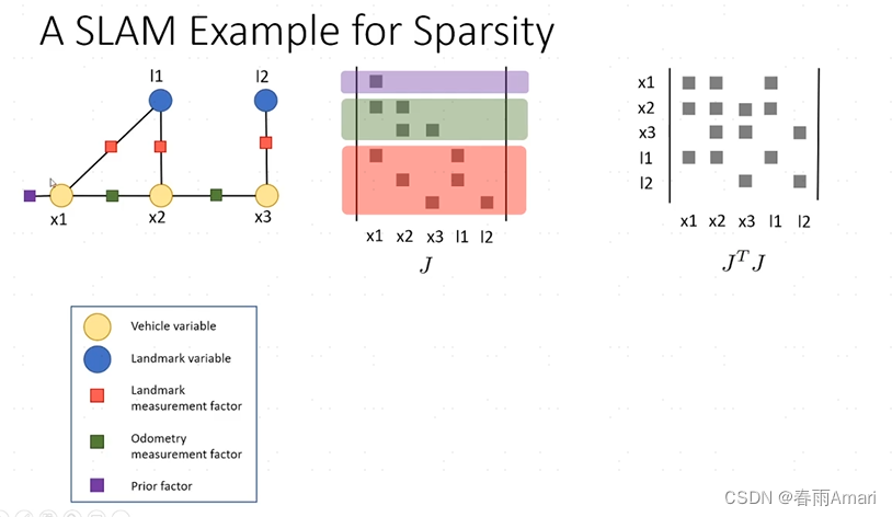
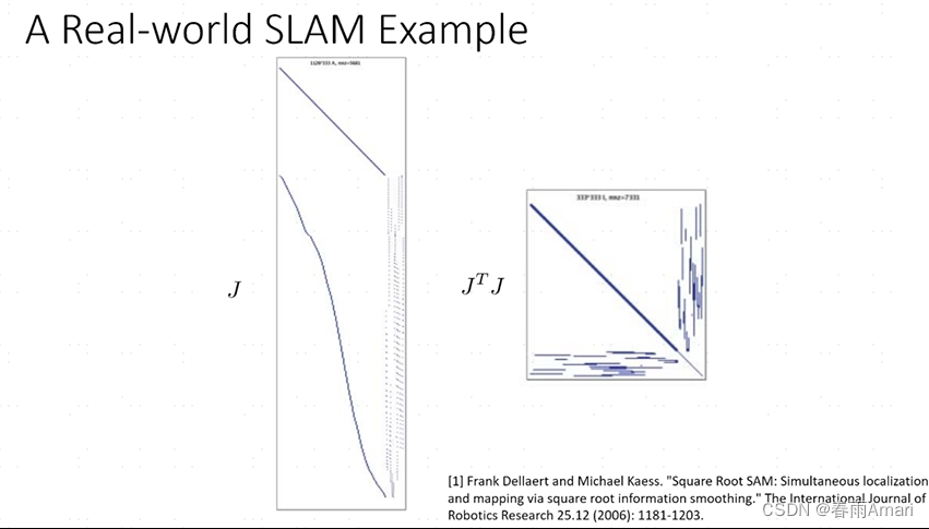
Each row of the Jacobian matrix in the above picture corresponds to a factor, and the matrix on the right is An information matrix. The Jacobian matrix obtained from the factor graph generated in reality is a sparse matrix. This is a good property and is very conducive to solving linear systems:
But this matrix The sparsity is related to the order of the variables. If the order is different, the sparsity of the matrix will be different, and the situation shown in the figure below will occur:
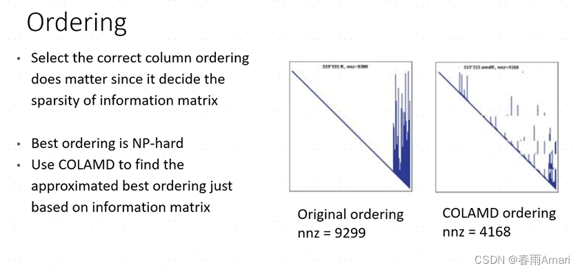
This situation is not conducive to solving the linear system. , so some algorithms are usually needed to reorder the information matrix to maintain its good sparsity. The currently more mature algorithm is COLAMD. Through the above description, we know how to solve a certain factor graph. However, the factor graph generated by common problems (such as SLAM problems) is incremental, and during the operation of the robot, the factor graph only changes a small part. If we decompose the factor graph from scratch to solve it, it is not conducive to The real-time nature of the system, so how to solve this problem? The following introduces how to do it in the paper isam. .
isam1 incremental QR decomposition
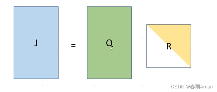
The QR decomposition for a given J is as shown below:
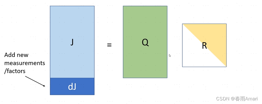
Now I want to add a few lines to J. The meaning of these lines is that when new elements are added to the factor graph When the nodes and factors are represented in the information matrix, there are just a few more rows. The question is how to get a new R without re-decomposing it.
The solution method is given in the paper, and the formula is as shown below:
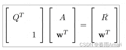
For adding a row (non-zero elements) below R, it becomes as shown below :
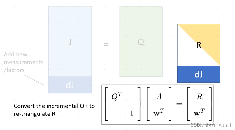
The solution is to turn R into a new upper triangular matrix through givens rotation:
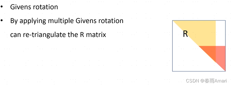
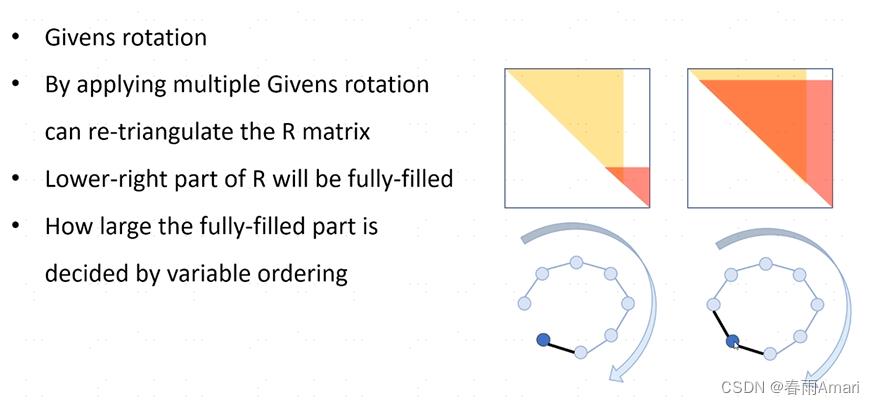
But as the factor increases, it will also bring about a The problem is that if the newly added factor only affects the factors at the previous moment, the matrix will still have good sparsity, but if the newly added factor is a loop, then givens rotation will affect all previous nodes, so that The R matrix becomes dense, as shown in the figure below
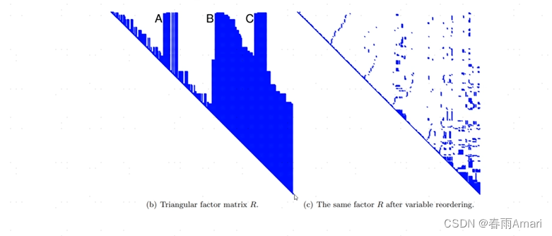
At this time, the problem of isam1 is reflected. After a certain period of time, the elements need to be reordered to make the dense matrix sparse. :
isam2
Here I briefly explain that isam2 converts the factor graph into a Bayesian network to solve. For specific articles, please refer to the paper. I have not studied it thoroughly myself. But I suggest that after you understand the process of solving factor graphs, don't look at the boring formulas anymore, it will hurt your brain. In fact, it is a tool for solving problems, so after understanding the problem, isn't it good to adjust the library?
Conclusion
The reason for writing this article is that I have been exposed to factor graph optimization early. For the factor graph optimization problem of the salm problem, I have never been able to figure out where this posterior probability is reflected. Now I finally understand. In fact, it is In the above process of deriving factors in exponential form, what is the Jacobian matrix? It turns out to be the first-order reciprocal of the matrix. So don’t be afraid of formulas when studying papers, because if you can’t understand the formulas, you really don’t understand, haha.